Analyze and visualize climatology
Overview
Teaching: 0 min
Exercises: 0 minQuestions
What is a climatology?
How to compare model outputs with a climatology?
Objectives
Learn about SPARC
Learn to compare CMIP6 model data with a climatology
What is a climatology?
A Climatology is a climate data series.
In this lesson, we will use climatological data issued from the Stratosphere-troposphere Processes And their Role in Climate project (SPARC) and in particular the Temperature and Zonal Wind Climatology.
SPARC Climatology
These data sets provide an updated climatology of zonal mean temperatures and winds covering altitudes 0-85 km. They are based on combining data from a variety of sources, and represent the time period 1992-1997 (SPARC Report No. 3, Randel et al 2002). https://www.sparc-climate.org/wp-content/uploads/sites/5/2017/12/SPARC_Report_No3_Dec2002_Climatologies.pdf
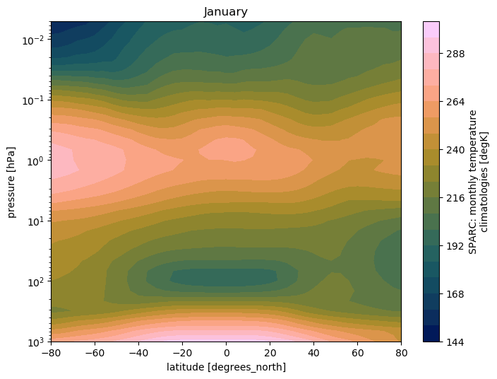
The zonal mean temperature climatology is derived using UK Met Office (METO) analyses over 1000-1.5 hPa, combined with Halogen Occultation Experiment (HALOE) temperature climatology over pressures 1.5-0.0046 hPa (~85 km).

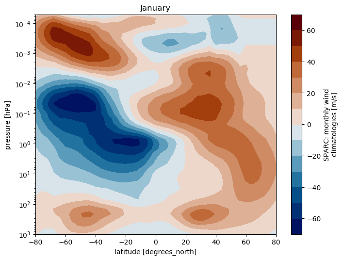
The monthly zonal wind climatology is derived from the UARS Reference Atmosphere Project (URAP), combining results from METO analyses with winds the UARS High Resolution Doppler Imager (HRDI). Details from the URAP winds are described in Swinbank and Ortland (2003).

NCAR’s Climate Data Guide (CDG) provides more information (search SPARC) including strengths and weaknesses of assorted data sets.
Plotting SPARC climatology
The SPARC climatology T and U is stored in a file called sparc.nc and can be found on the Jupyterhub.
In the Jupyterhub Terminal:
cd $HOME/shared-tacco-ns1004k/SPARC
ls
sparc.nc
Plotting SPARC climatology using python
Open SPARC climatology netCDF file
import xarray as xr
import matplotlib as mpl
import matplotlib.pyplot as plt
import numpy as np
import calendar

mpl.rcParams['figure.figsize'] = [8., 6.]

filename = 'shared-tacco-ns1004k/SPARC/sparc.nc'
ds = xr.open_dataset(filename)
ds
<xarray.Dataset>
Dimensions:   (lat: 41, lev_temp: 33, lev_wind: 46, month: 12)
Coordinates:
  * lev_wind  (lev_wind) float32 1000.0 681.29193 ... 3.1622778e-05
  * lat       (lat) float32 -80.0 -76.0 -72.0 -68.0 ... 68.0 72.0 76.0 80.0
  * month     (month) int32 1 2 3 4 5 6 7 8 9 10 11 12
  * lev_temp  (lev_temp) float32 1000.0 681.29193 ... 0.006812923 0.004641587
Data variables:
    WIND      (lev_wind, lat, month) float32 ...
    TEMP      (lev_temp, lat, month) float32 ...
Attributes:
    creation_date:  Tue Feb 21 09:23:03 CET 2017
    creator:        D. Shea, NCAR
    Conventions:    None
    referencese:    \nRandel, W.J. et al., (2004)                            ...
    WWW_data:       http://www.sparc-climate.org/data-center/data-access/refe...
    WWW:            http://www.sparc-climate.org/
    README:         ftp://sparc-ftp1.ceda.ac.uk/sparc/ref_clim/randel/temp_wi...
    title:          SPARC Intercomparison of Middle Atmosphere Climatologies
SPARC climatology: Plot Temperature
#import color maps
%run shared-tacco-ns1004k/scripts/load_cmap.ipynb

# plot for January (month=0)
ds.TEMP.isel(month=0).plot.contourf(cmap=load_cmap('batlow'),
                                   levels=20)

plt.title(calendar.month_name[1])
plt.ylim(plt.ylim()[::-1])
plt.yscale('log')
plt.ylim(top=0.005)
plt.ylim(bottom=1000.)
plt.xlim(left=ds.TEMP.lat.min())
plt.xlim(right=ds.TEMP.lat.max())
SPARC climatology: Plot zonal wind
ds.WIND.isel(month=0).plot.contourf(cmap=load_cmap('vik'),
                                   levels=15)

plt.title(calendar.month_name[1])
plt.ylim(plt.ylim()[::-1])
plt.yscale('log')
plt.ylim(top=5.0e-5)
plt.ylim(bottom=1000.)
plt.xlim(left=ds.TEMP.lat.min())
plt.xlim(right=ds.TEMP.lat.max())
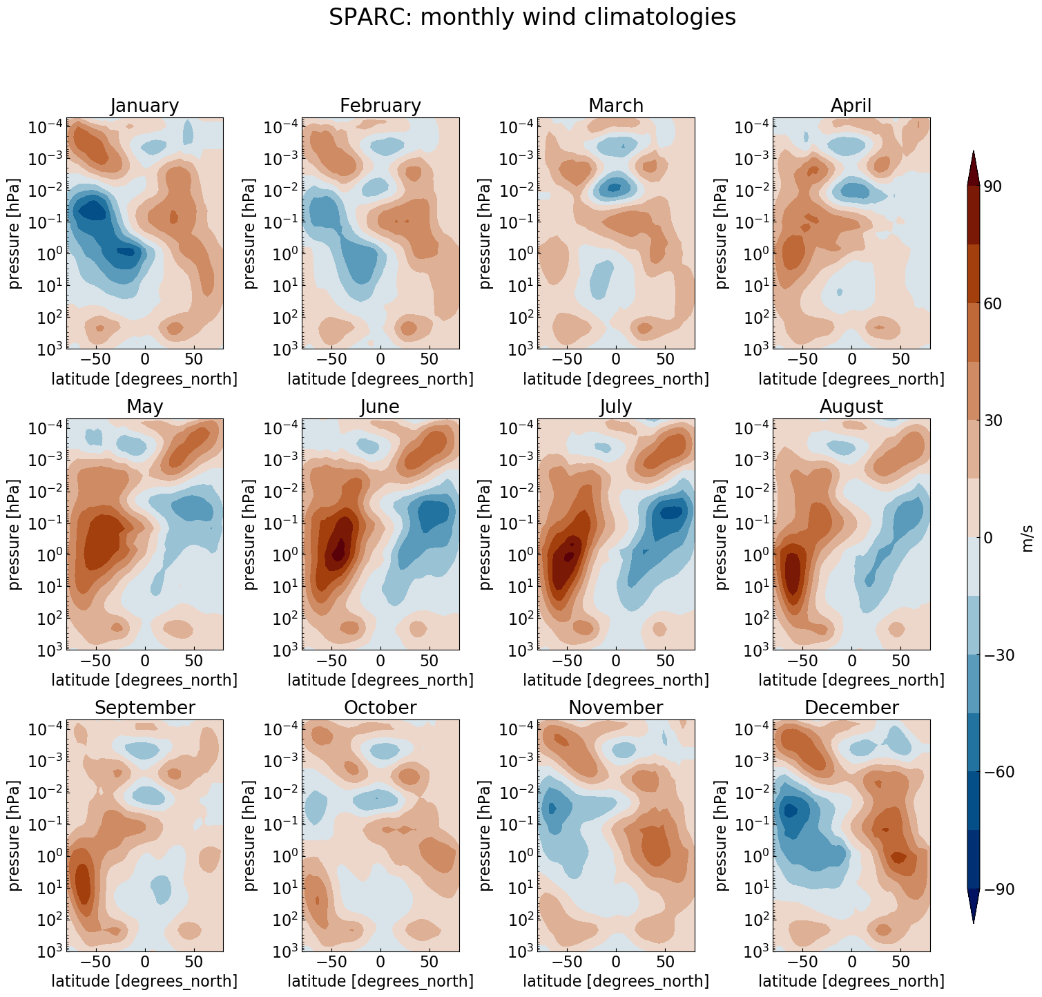
Multiple plots
To generate 12 subplots (one per month) for the zonal wind and temperature climatology, we can use the Python range(start, stop[, step]) function (remember that the range of integers ends at stop - 1):
import xarray as xr
import matplotlib as mpl
import matplotlib.pyplot as plt
import numpy as np
import calendar

fig = plt.figure(figsize=[18,16])
for month in range(1,13):
    ax = fig.add_subplot(3, 4, month)  # specify number of rows and columns, and axis

    ax.set_title(label = calendar.month_name[month])

fig.suptitle(ds.WIND.attrs['long_name'], fontsize=22)

# Add shared colorbar:
fig.subplots_adjust(right=0.82, wspace=0.5, hspace=0.3) # adjust subplots so we keep a bit of space on the right for the colorbar
cbar_ax = fig.add_axes([0.85, 0.15, 0.01, 0.7]) # Specify where to place the colorbar
#fig.colorbar(<handle of your contour plot here>, cax=cbar_ax, label=ds.WIND.attrs['units']) # Add a colorbar to the figure
This allows you to plot, e.g., the zonal wind like this:
Make a multiple plot for the SPARC temperature
Make the same kind of multiple plot but for the temperature instead.
Home-assignment: Visualize and compare CMIP6 model data to the SPARC climatology
Now that we are familiar with the SPARC climatology, we are ready to analyze CMIP6 model data and make comparison with it. This is the goal of the first exercise you will have to fulfill.
To help you we give some hints for a methodology you can follow (please note that there is not one unique way to analyze and plot, and you should feel free to divert from the methodology given), and will assist you during the class.
Methodology
Which data to analyze and why?
You can analyze many variables from the control run to check its validity but at least temperature and zonal wind, as these two variables are the ones contained in the SPARC climatology.
You have a lot of model data at hand. Discuss with your fellow students and tutors which CMIP6 data it makes sense to compare to the SPARC climatology.
Useful Python code
If the data you need are separated into different files, you can load several files at once and concatenate (or combine) them.
# load multiple specified files
path = 'shared-tacco-ns1004k-cmip-betzy/NCAR/CESM2/historical/r10i1p1f1/Amon/ua/gn/latest/'
files = [path+'ua_Amon_CESM2_historical_r10i1p1f1_gn_195001-199912.nc',
         path+'ua_Amon_CESM2_historical_r10i1p1f1_gn_200001-201412.nc']
files
['shared-tacco-ns1004k-cmip-betzy/NCAR/CESM2/historical/r10i1p1f1/Amon/ua/gn/latest/ua_Amon_CESM2_historical_r10i1p1f1_gn_195001-199912.nc',
 'shared-tacco-ns1004k-cmip-betzy/NCAR/CESM2/historical/r10i1p1f1/Amon/ua/gn/latest/ua_Amon_CESM2_historical_r10i1p1f1_gn_200001-201412.nc']
You can also use wildcards (i.e. “*”) for loading many files.
import glob
import os

# load loads of files
path = 'shared-tacco-ns1004k-cmip-betzy/NCAR/CESM2/historical/r10i1p1f1/Amon/ua/gn/latest/'
files =  glob.glob(os.path.join(path, 'ua_Amon_CESM2_historical_r10i1p1f1_gn_*'))
# sort files so they appear by year/month
files.sort()
files
['shared-tacco-ns1004k-cmip-betzy/NCAR/CESM2/historical/r10i1p1f1/Amon/ua/gn/latest/ua_Amon_CESM2_historical_r10i1p1f1_gn_185001-189912.nc',
 'shared-tacco-ns1004k-cmip-betzy/NCAR/CESM2/historical/r10i1p1f1/Amon/ua/gn/latest/ua_Amon_CESM2_historical_r10i1p1f1_gn_190001-194912.nc',
 'shared-tacco-ns1004k-cmip-betzy/NCAR/CESM2/historical/r10i1p1f1/Amon/ua/gn/latest/ua_Amon_CESM2_historical_r10i1p1f1_gn_195001-199912.nc',
 'shared-tacco-ns1004k-cmip-betzy/NCAR/CESM2/historical/r10i1p1f1/Amon/ua/gn/latest/ua_Amon_CESM2_historical_r10i1p1f1_gn_200001-201412.nc']
Now that we have a list of the file names, we can load all files at once into the same xarray dataset using xarray.open_mfdataset(), which knows to concatenate the files in the time dimension.
import xarray as xr

ds = xr.open_mfdataset(files, combine='by_coords')
ds
<xarray.Dataset>
Dimensions:    (lat: 192, lon: 288, nbnd: 2, plev: 19, time: 780)
Coordinates:
  * lon        (lon) float64 0.0 1.25 2.5 3.75 5.0 ... 355.0 356.2 357.5 358.8
  * plev       (plev) float64 1e+05 9.25e+04 8.5e+04 7e+04 ... 1e+03 500.0 100.0
  * lat        (lat) float64 -90.0 -89.06 -88.12 -87.17 ... 88.12 89.06 90.0
  * time       (time) object 1950-01-15 12:00:00 ... 2014-12-15 12:00:00
Dimensions without coordinates: nbnd
Data variables:
    ua         (time, plev, lat, lon) float32 dask.array<chunksize=(600, 19, 192, 288), meta=np.ndarray>
    time_bnds  (time, nbnd) object dask.array<chunksize=(600, 2), meta=np.ndarray>
    lat_bnds   (time, lat, nbnd) float64 dask.array<chunksize=(600, 192, 2), meta=np.ndarray>
    lon_bnds   (time, lon, nbnd) float64 dask.array<chunksize=(600, 288, 2), meta=np.ndarray>
Attributes:
    Conventions:            CF-1.7 CMIP-6.2
    activity_id:            CMIP
    branch_method:          standard
    branch_time_in_child:   674885.0
    branch_time_in_parent:  306600.0
    case_id:                24
    cesm_casename:          b.e21.BHIST.f09_g17.CMIP6-historical.010
    contact:                cesm_cmip6@ucar.edu
    creation_date:          2019-03-12T05:37:46Z
    data_specs_version:     01.00.29
    experiment:             Simulation of recent past (1850 to 2014). Impose ...
    experiment_id:          historical
    external_variables:     areacella
    forcing_index:          1
    frequency:              mon
    further_info_url:       https://furtherinfo.es-doc.org/CMIP6.NCAR.CESM2.h...
    grid:                   native 0.9x1.25 finite volume grid (192x288 latxlon)
    grid_label:             gn
    initialization_index:   1
    institution:            National Center for Atmospheric Research, Climate...
    institution_id:         NCAR
    license:                CMIP6 model data produced by <The National Center...
    mip_era:                CMIP6
    model_doi_url:          https://doi.org/10.5065/D67H1H0V
    nominal_resolution:     100 km
    parent_activity_id:     CMIP
    parent_experiment_id:   piControl
    parent_mip_era:         CMIP6
    parent_source_id:       CESM2
    parent_time_units:      days since 0001-01-01 00:00:00
    parent_variant_label:   r1i1p1f1
    physics_index:          1
    product:                model-output
    realization_index:      10
    realm:                  atmos
    source:                 CESM2 (2017): atmosphere: CAM6 (0.9x1.25 finite v...
    source_id:              CESM2
    source_type:            AOGCM BGC
    sub_experiment:         none
    sub_experiment_id:      none
    table_id:               Amon
    tracking_id:            hdl:21.14100/08811120-5c62-417b-97dd-a477ad5820ef
    variable_id:            ua
    variant_info:           CMIP6 20th century experiments (1850-2014) with C...
    variant_label:          r10i1p1f1
We can apply functions to the xarray.Dataset. For example, we can first group the data by month and then average over each of these months.
dy = ds.groupby('time.month').mean('time')
dy
<xarray.Dataset>
Dimensions:   (bnds: 2, lat: 192, lon: 384, month: 12, plev: 19)
Coordinates:
  * lat       (lat) float64 -89.28 -88.36 -87.42 -86.49 ... 87.42 88.36 89.28
  * plev      (plev) float64 1e+05 9.25e+04 8.5e+04 7e+04 ... 1e+03 500.0 100.0
  * lon       (lon) float64 0.0 0.9375 1.875 2.812 ... 356.2 357.2 358.1 359.1
  * month     (month) int64 1 2 3 4 5 6 7 8 9 10 11 12
Dimensions without coordinates: bnds
Data variables:
    lat_bnds  (month, lat, bnds) float64 dask.array<chunksize=(1, 192, 2), meta=np.ndarray>
    lon_bnds  (month, lon, bnds) float64 dask.array<chunksize=(1, 384, 2), meta=np.ndarray>
    ua        (month, plev, lat, lon) float32 dask.array<chunksize=(1, 19, 192, 384), meta=np.ndarray>
Important note
As we are using xarray, computations are deferred, which means that we still haven’t loaded much in memory. Computations will be done when we need to access the data, for example by plotting it.
If you want to save your results in a new netcdf file, you can do this with the to_netcdf xarray method:
dy[['ua']].to_netcdf("ua_Amon_MPI-ESM1-2-HR_historical_r1i1p1f1_gn_201001-201412_clim.nc")
You can then load your saved files back when you need them later, without having to repeat your data processing.
ds = xr.open_dataset("ua_Amon_MPI-ESM1-2-HR_historical_r1i1p1f1_gn_201001-201412_clim.nc")
You are now ready to visualize zonal wind and temperature from CMIP6 model data and start the home-assignment where you will compare this with the SPARC climatology!
Home-assignment
How well does your model represent the SPARC climatology?To answer this question:
- Write a Python 3 Jupyter notebook and name it exercise_sparc_vs_YOUR-MODEL-NAME_YOURNAME.ipynb where you need to replace YOUR-MODEL-NAME by the model you choose to analyze and YOURNAME by your name!
- Follow the methodology given in this lesson and compare the results from your model data and the SPARC climatology.
- Your answer should contain plots of the climatologies, an explanation of what you have plotted and why, and a brief dicsussion of how the climatologies compare.
- Send it by email to the instructors/teachers. We will discuss your results in next Monday’s model practical.
Deadline
Hand in the exercise by 10:00 on Monday March 6, 2023!Key Points
SPARC
climatology