Some tips with xarray and pandas

• We have massively different levels here

• Try to make some aims for technical skills you can learn!

  • If you are beginning with python → learn the basics

  • If you are good at basic python → learn new packages and tricks

  • If you know all the packages → improve your skills with producing your own software, organising your code etc.

  • If you don’t know git and github → get better at this!

• Learn from each other!

• Every time I taught on this course, I learned something!

• AI is a real game changer and we are figuring out together how to use it well!

  • Especially great to give us feedback on this.

Please feel free to come with suggestions and extra input as we go!

CHANGE: Etherpad for the course

Note to Sara: do menti

Jupyter notebooks:

Jupyter is an interactive computing environment that allows users to write, run, and document code in a single interface, typically using notebooks that combine live code, text, equations, and visualizations. It supports multiple programming languages (like Python, R, and Julia) and is widely used in data science, research, and education for reproducible analysis and exploration.

a=1
import numpy as np
a

1

• cells can be markdown or code

• run cell by shift+enter, cmd+enter, ctrl+enter

• Kernel: You can restart, interrupt etc.

• Tricks:

  • mark multiple places at the same time

  • cmd or ctr + D: select same snippet.

  • Escape to move out of cell

    • Once out of cell mode, you can copy (c), paste (v), insert cell above (a), incert cell below (b) etc.

• Contextual help: cmd+i or ctrl+i

.

.

.

.

.

What are pandas and xarray?

• Pandas → like a spreadsheet 2D data with columns and rows

• xarray → like pandas, but in N dimensions

• Use the functionality these packages gives you! Will help you avoid mistakes. Try to get as good as possible :)

Pandas

(Source: https://www.geeksforgeeks.org/python-pandas-dataframe/)

Xarray

(Source: https://docs.xarray.dev/)

.

.

.

.

.

1. Import python packages

import xarray as xr
xr.set_options(display_style='html')
import intake
import cftime
import matplotlib.pyplot as plt
import cartopy.crs as ccrs
import numpy as np
import pandas as pd
import datetime
import seaborn as sns
%matplotlib inline

2. Pandas basics:

Can read a range of data formats, e.g.

pd.read_csv('filename.csv')
pd.read_excel('filename')
pd.read_sql('filename')

See overview: https://pandas.pydata.org/pandas-docs/stable/user_guide/io.html

#fn = '~/shared-craas2-ns9988k-ns9252k/escience2025/data/group3/eScience2024/zeppelin-ebc-2015-2019-1.csv'
fn = '~/shared-clinfra-ns12127k-ns9252k/eScience-courses/escience2024/data/data_group4/zeppelin-ebc-2015-2019-1.csv'

Read in as a DataFrame

import pandas as pd

df = pd.read_csv(fn, index_col=0, parse_dates=True )
df

	CVI_status	BC_cvi	z	BC_tot	flag	visibility
time
2015-11-13 00:00:00	off	0.00	0.30583	0.04	bad	34596.2
2015-11-13 00:01:00	off	0.00	0.43400	0.02	bad	34481.7
2015-11-13 00:02:00	off	0.04	0.53317	0.01	bad	34572.3
2015-11-13 00:03:00	off	0.05	0.60250	0.02	bad	34061.8
2015-11-13 00:04:00	off	-0.01	1.16433	0.02	bad	34461.8
...	...	...	...	...	...	...
2019-11-15 10:30:00	off	0.02	1.14300	0.02	good	36983.4
2019-11-15 10:31:00	off	0.00	1.34233	0.01	good	38964.4
2019-11-15 10:32:00	off	0.05	0.68667	-0.00	good	45981.7
2019-11-15 10:33:00	off	-0.02	1.00450	-0.00	good	48805.2
2019-11-15 10:34:00	off	0.04	0.86300	0.01	good	47112.9

2107355 rows × 6 columns

Select a column:

One column is called a Series

df['BC_cvi']

time
2015-11-13 00:00:00    0.00
2015-11-13 00:01:00    0.00
2015-11-13 00:02:00    0.04
2015-11-13 00:03:00    0.05
2015-11-13 00:04:00   -0.01
                       ... 
2019-11-15 10:30:00    0.02
2019-11-15 10:31:00    0.00
2019-11-15 10:32:00    0.05
2019-11-15 10:33:00   -0.02
2019-11-15 10:34:00    0.04
Name: BC_cvi, Length: 2107355, dtype: float64

Select data in general:

Several ways to do this:

df.loc[<from_index>: <to_index>, <from_column>:<to_column>]

df.loc['2016-01-01':'2016-01-02', 'CVI_status':'BC_cvi']#['BC_cvi']

	CVI_status	BC_cvi
time
2016-01-01 00:00:00	off	0.13
2016-01-01 00:01:00	off	0.11
2016-01-01 00:02:00	off	0.03
2016-01-01 00:03:00	off	0.03
2016-01-01 00:04:00	off	0.00
...	...	...
2016-01-02 23:55:00	off	0.02
2016-01-02 23:56:00	off	0.00
2016-01-02 23:57:00	off	0.12
2016-01-02 23:58:00	off	0.00
2016-01-02 23:59:00	off	0.07

2880 rows × 2 columns

The same, but using indexes:

df.iloc[0:5, 0:2]#['BC_cvi']

	CVI_status	BC_cvi
time
2015-11-13 00:00:00	off	0.00
2015-11-13 00:01:00	off	0.00
2015-11-13 00:02:00	off	0.04
2015-11-13 00:03:00	off	0.05
2015-11-13 00:04:00	off	-0.01

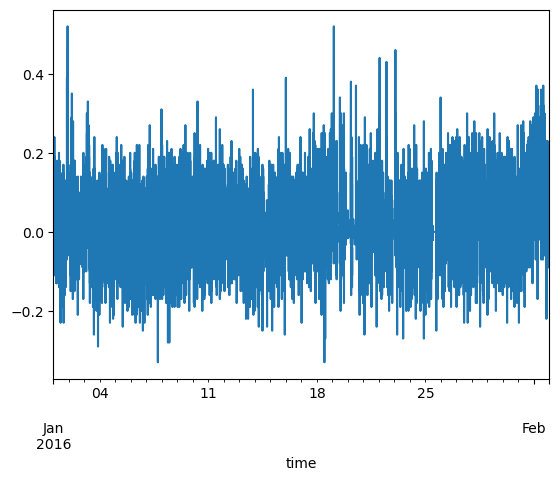
Plot something simple:

df.loc['2016-01-01':'2016-02-01','BC_cvi'].plot()

<Axes: xlabel='time'>

Save your dataframe:

df.to_csv('my_new_dataset.csv')

3. Xarray and netcdf

3.1 Reading in the data from a netcdf file:

Netcdf format:

• NetCDF (Network Common Data Form) is a widely used, platform-independent file format designed for array-oriented scientific data.

• It is self-describing, meaning metadata (e.g., units, descriptions) is stored alongside the data.

• Supports multidimensional data structures, such as time-varying grids (e.g., time, latitude, longitude, level).

• Commonly used in earth and atmospheric sciences for storing model outputs, reanalyses, and satellite data. Developed at UCAR.

• Organizes content into:

  • Dimensions (e.g., time, lat, lon)

  • Variables (e.g., temperature, pressure)

  • Attributes (e.g., units, standard names, conventions)

• Enables efficient storage and retrieval, even for very large datasets.

• Supported by many scientific tools and libraries including xarray, netCDF4, NCO, and CDO.

• Ideal for interoperability, reproducibility, and long-term data archiving.

NetCDF + xarray = <3

Xarray is a Python library designed to work with multi-dimensional arrays and datasets, particularly those used in earth sciences, climate science, and atmospheric science. It builds upon and extends the functionality of NumPy, Pandas, and NetCDF, providing a high-level interface for working with labeled, multi-dimensional data.

.

.

.

.

.

Open dataset

• Use xarray python package to analyze netCDF dataset

• open_dataset allows to get all the metadata without loading data into memory.

• with xarray, we only load into memory what is needed.

path='filename.nc'
ds = xr.open_dataset(path)

Opening multiple files:

list_of_files = [
    'file1.nc',
    'file2.nc'
]
xr.open_mfdataset(list_of_files, concat_dim='time',combine='by_coords')

Example:

(I’ve gone hunting in your data folders)

f1 = '~/shared-clinfra-ns12127k-ns9252k/eScience-courses/escience2025/data/group6/CMIP6/abrupt-4xCO2/rlut_Amon_CAMS-CSM1-0_abrupt-4xCO2_r1i1p1f1_gn.nc'
#f2 = '~/shared-craas2-ns9988k-ns9252k/escience2025/data/group6/CMIP6/abrupt-4xCO2/rsut_Amon_CAMS-CSM1-0_abrupt-4xCO2_r1i1p1f1_gn.nc'
f2 = '~/shared-clinfra-ns12127k-ns9252k/eScience-courses/escience2025/data/group6/CMIP6/abrupt-4xCO2/rsut_Amon_CAMS-CSM1-0_abrupt-4xCO2_r1i1p1f1_gn.nc'

Open one file:

xr.open_dataset(f1)

/opt/conda/envs/pangeo/lib/python3.12/site-packages/dask/config.py:786: FutureWarning: Dask configuration key 'distributed.p2p.disk' has been deprecated; please use 'distributed.p2p.storage.disk' instead
  warnings.warn(

<xarray.Dataset> Size: 369MB
Dimensions:  (time: 1800, lat: 160, lon: 320)
Coordinates:
  * time     (time) object 14kB 0001-01-01 00:00:00 ... 0150-12-01 00:00:00
  * lat      (lat) float64 1kB -89.14 -88.03 -86.91 -85.79 ... 86.91 88.03 89.14
  * lon      (lon) float64 3kB 0.0 1.125 2.25 3.375 ... 355.5 356.6 357.8 358.9
Data variables:
    rlut     (time, lat, lon) float32 369MB ...
Attributes: (12/50)
    CDI:                    Climate Data Interface version 2.0.5 (https://mpi...
    Conventions:            CF-1.7 CMIP-6.2
    source:                 CAMS_CSM 1.0 (2016): \naerosol: none\natmos: ECHA...
    institution:            Chinese Academy of Meteorological Sciences, Beiji...
    activity_id:            CMIP
    branch_method:          Standard
    ...                     ...
    tracking_id:            hdl:21.14100/73320c27-d385-493c-9674-1470acacb8ed
    variable_id:            rlut
    variant_label:          r1i1p1f1
    license:                CMIP6 model data produced by Lawrence Livermore P...
    cmor_version:           3.4.0
    CDO:                    Climate Data Operators version 2.0.5 (https://mpi...

xarray.Dataset

• Dimensions:
  • time: 1800
  • lat: 160
  • lon: 320
• Coordinates: (3)
  • time
    (time)
    object
    0001-01-01 00:00:00 ... 0150-12-...

    array([cftime.DatetimeNoLeap(1, 1, 1, 0, 0, 0, 0, has_year_zero=True),
           cftime.DatetimeNoLeap(1, 2, 1, 0, 0, 0, 0, has_year_zero=True),
           cftime.DatetimeNoLeap(1, 3, 1, 0, 0, 0, 0, has_year_zero=True), ...,
           cftime.DatetimeNoLeap(150, 10, 1, 0, 0, 0, 0, has_year_zero=True),
           cftime.DatetimeNoLeap(150, 11, 1, 0, 0, 0, 0, has_year_zero=True),
           cftime.DatetimeNoLeap(150, 12, 1, 0, 0, 0, 0, has_year_zero=True)],
          shape=(1800,), dtype=object)

  • lat
    (lat)
    float64
    -89.14 -88.03 ... 88.03 89.14

    standard_name :

    latitude

    long_name :

    Latitude

    units :

    degrees_north

    axis :

    Y

    bounds :

    lat_bnds

    array([-89.141519, -88.029429, -86.910771, -85.790629, -84.669924, -83.548947,
           -82.427818, -81.306595, -80.18531 , -79.063982, -77.942624, -76.821243,
           -75.699844, -74.578432, -73.457008, -72.335576, -71.214136, -70.09269 ,
           -68.97124 , -67.849784, -66.728326, -65.606864, -64.485399, -63.363932,
           -62.242462, -61.120991, -59.999518, -58.878044, -57.756569, -56.635092,
           -55.513614, -54.392135, -53.270655, -52.149175, -51.027694, -49.906212,
           -48.784729, -47.663246, -46.541763, -45.420279, -44.298794, -43.177309,
           -42.055824, -40.934338, -39.812852, -38.691366, -37.56988 , -36.448393,
           -35.326906, -34.205418, -33.083931, -31.962443, -30.840955, -29.719467,
           -28.597979, -27.476491, -26.355002, -25.233514, -24.112025, -22.990536,
           -21.869047, -20.747558, -19.626069, -18.50458 , -17.383091, -16.261601,
           -15.140112, -14.018622, -12.897133, -11.775643, -10.654153,  -9.532664,
            -8.411174,  -7.289684,  -6.168194,  -5.046704,  -3.925215,  -2.803725,
            -1.682235,  -0.560745,   0.560745,   1.682235,   2.803725,   3.925215,
             5.046704,   6.168194,   7.289684,   8.411174,   9.532664,  10.654153,
            11.775643,  12.897133,  14.018622,  15.140112,  16.261601,  17.383091,
            18.50458 ,  19.626069,  20.747558,  21.869047,  22.990536,  24.112025,
            25.233514,  26.355002,  27.476491,  28.597979,  29.719467,  30.840955,
            31.962443,  33.083931,  34.205418,  35.326906,  36.448393,  37.56988 ,
            38.691366,  39.812852,  40.934338,  42.055824,  43.177309,  44.298794,
            45.420279,  46.541763,  47.663246,  48.784729,  49.906212,  51.027694,
            52.149175,  53.270655,  54.392135,  55.513614,  56.635092,  57.756569,
            58.878044,  59.999518,  61.120991,  62.242462,  63.363932,  64.485399,
            65.606864,  66.728326,  67.849784,  68.97124 ,  70.09269 ,  71.214136,
            72.335576,  73.457008,  74.578432,  75.699844,  76.821243,  77.942624,
            79.063982,  80.18531 ,  81.306595,  82.427818,  83.548947,  84.669924,
            85.790629,  86.910771,  88.029429,  89.141519])

  • lon
    (lon)
    float64
    0.0 1.125 2.25 ... 357.8 358.9

    standard_name :

    longitude

    long_name :

    Longitude

    units :

    degrees_east

    axis :

    X

    bounds :

    lon_bnds

    array([  0.   ,   1.125,   2.25 , ..., 356.625, 357.75 , 358.875], shape=(320,))

• Data variables: (1)
  • rlut
    (time, lat, lon)
    float32
    ...

    standard_name :

    toa_outgoing_longwave_flux

    long_name :

    TOA Outgoing Longwave Radiation

    units :

    W m-2

    CDI_grid_type :

    gaussian

    CDI_grid_num_LPE :

    80

    comment :

    at the top of the atmosphere (to be compared with satellite measurements)

    original_name :

    trad0

    cell_methods :

    area: time: mean

    cell_measures :

    area: areacella

    history :

    2019-07-01T12:39:23Z altered by CMOR: Inverted axis: lat.

    [92160000 values with dtype=float32]

• Attributes: (50)

  CDI :

  Climate Data Interface version 2.0.5 (https://mpimet.mpg.de/cdi)

  Conventions :

  CF-1.7 CMIP-6.2

  source :

  CAMS_CSM 1.0 (2016): aerosol: none atmos: ECHAM5_CAMS (T106; 320 x 160 longitude/latitude; 31 levels; top level 10 mb) atmosChem: none land: CoLM 1.0 landIce: none ocean: MOM4 (tripolar; 360 x 200 longitude/latitude, primarily 1deg latitude/longitude, down to 1/3deg within 30deg of the equatorial tropics; 50 levels; top grid cell 0-10 m) ocnBgchem: none seaIce: SIS 1.0

  institution :

  Chinese Academy of Meteorological Sciences, Beijing 100081, China

  activity_id :

  CMIP

  branch_method :

  Standard

  branch_time_in_child :

  0.0

  branch_time_in_parent :

  3030.0

  contact :

  Dr. Xinyao Rong (rongxy@cma.gov.cn)

  creation_date :

  2019-07-01T12:39:23Z

  data_specs_version :

  01.00.30

  description :

  DECK: abrupt4xCO2

  experiment :

  abrupt quadrupling of CO2

  experiment_id :

  abrupt-4xCO2

  external_variables :

  areacella

  forcing_index :

  1

  frequency :

  mon

  further_info_url :

  https://furtherinfo.es-doc.org/CMIP6.CAMS.CAMS-CSM1-0.abrupt-4xCO2.none.r1i1p1f1

  grid :

  T106

  grid_label :

  gn

  history :

  Fri Mar 21 19:16:15 2025: cdo -O -s -mergetime /pool/data/CMIP6/data/CMIP/CAMS/CAMS-CSM1-0/abrupt-4xCO2/r1i1p1f1/Amon/rlut/gn/v20190708/rlut_Amon_CAMS-CSM1-0_abrupt-4xCO2_r1i1p1f1_gn_303001-317912.nc rlut_Amon_CAMS-CSM1-0_abrupt-4xCO2_r1i1p1f1_gn.nc 2019-07-01T12:31:20Z ;rewrote data to be consistent with CMIP for variable hfls found in table Amon.; Output from CAMS-CSM1-0

  initialization_index :

  1

  institution_id :

  CAMS

  mip_era :

  CMIP6

  nominal_resolution :

  100 km

  parent_activity_id :

  CMIP

  parent_experiment_id :

  piControl

  parent_mip_era :

  CMIP6

  parent_source_id :

  CAMS-CSM1-0

  parent_time_units :

  days since 3030-01-01

  parent_variant_label :

  r1i1p1f1

  physics_index :

  1

  product :

  model-output

  realization_index :

  1

  realm :

  atmos

  references :

  Model described by Rong et al (J. Meteoro. Res., 2019, 576-591).

  run_variant :

  forcing: GHG

  source_id :

  CAMS-CSM1-0

  source_type :

  AOGCM

  sub_experiment :

  none

  sub_experiment_id :

  none

  table_id :

  Amon

  table_info :

  Creation Date:(30 April 2019) MD5:cc2ae51c23960ce127b4d68ab3d8ac87

  title :

  CAMS-CSM1-0 output prepared for CMIP6

  tracking_id :

  hdl:21.14100/73320c27-d385-493c-9674-1470acacb8ed

  variable_id :

  rlut

  variant_label :

  r1i1p1f1

  license :

  CMIP6 model data produced by Lawrence Livermore PCMDI is licensed under a Creative Commons Attribution ShareAlike 4.0 International License (https://creativecommons.org/licenses). Consult https://pcmdi.llnl.gov/CMIP6/TermsOfUse for terms of use governing CMIP6 output, including citation requirements and proper acknowledgment. Further information about this data, including some limitations, can be found via the further_info_url (recorded as a global attribute in this file) and at https:///pcmdi.llnl.gov/. The data producers and data providers make no warranty, either express or implied, including, but not limited to, warranties of merchantability and fitness for a particular purpose. All liabilities arising from the supply of the information (including any liability arising in negligence) are excluded to the fullest extent permitted by law.

  cmor_version :

  3.4.0

  CDO :

  Climate Data Operators version 2.0.5 (https://mpimet.mpg.de/cdo)

Open multiple files:

ds1 = xr.open_mfdataset([f1, f2])

3.1 Check how your dataset looks

Notice:

• Coordinates

• Data variables (each with assigned coordinates)

• Attributes

ds1

<xarray.Dataset> Size: 737MB
Dimensions:  (time: 1800, lat: 160, lon: 320)
Coordinates:
  * time     (time) object 14kB 0001-01-01 00:00:00 ... 0150-12-01 00:00:00
  * lat      (lat) float64 1kB -89.14 -88.03 -86.91 -85.79 ... 86.91 88.03 89.14
  * lon      (lon) float64 3kB 0.0 1.125 2.25 3.375 ... 355.5 356.6 357.8 358.9
Data variables:
    rlut     (time, lat, lon) float32 369MB dask.array<chunksize=(1, 160, 320), meta=np.ndarray>
    rsut     (time, lat, lon) float32 369MB dask.array<chunksize=(1, 160, 320), meta=np.ndarray>
Attributes: (12/50)
    CDI:                    Climate Data Interface version 2.0.5 (https://mpi...
    Conventions:            CF-1.7 CMIP-6.2
    source:                 CAMS_CSM 1.0 (2016): \naerosol: none\natmos: ECHA...
    institution:            Chinese Academy of Meteorological Sciences, Beiji...
    activity_id:            CMIP
    branch_method:          Standard
    ...                     ...
    tracking_id:            hdl:21.14100/73320c27-d385-493c-9674-1470acacb8ed
    variable_id:            rlut
    variant_label:          r1i1p1f1
    license:                CMIP6 model data produced by Lawrence Livermore P...
    cmor_version:           3.4.0
    CDO:                    Climate Data Operators version 2.0.5 (https://mpi...

xarray.Dataset

• Dimensions:
  • time: 1800
  • lat: 160
  • lon: 320
• Coordinates: (3)
  • time
    (time)
    object
    0001-01-01 00:00:00 ... 0150-12-...

    array([cftime.DatetimeNoLeap(1, 1, 1, 0, 0, 0, 0, has_year_zero=True),
           cftime.DatetimeNoLeap(1, 2, 1, 0, 0, 0, 0, has_year_zero=True),
           cftime.DatetimeNoLeap(1, 3, 1, 0, 0, 0, 0, has_year_zero=True), ...,
           cftime.DatetimeNoLeap(150, 10, 1, 0, 0, 0, 0, has_year_zero=True),
           cftime.DatetimeNoLeap(150, 11, 1, 0, 0, 0, 0, has_year_zero=True),
           cftime.DatetimeNoLeap(150, 12, 1, 0, 0, 0, 0, has_year_zero=True)],
          shape=(1800,), dtype=object)

  • lat
    (lat)
    float64
    -89.14 -88.03 ... 88.03 89.14

    standard_name :

    latitude

    long_name :

    Latitude

    units :

    degrees_north

    axis :

    Y

    bounds :

    lat_bnds

    array([-89.141519, -88.029429, -86.910771, -85.790629, -84.669924, -83.548947,
           -82.427818, -81.306595, -80.18531 , -79.063982, -77.942624, -76.821243,
           -75.699844, -74.578432, -73.457008, -72.335576, -71.214136, -70.09269 ,
           -68.97124 , -67.849784, -66.728326, -65.606864, -64.485399, -63.363932,
           -62.242462, -61.120991, -59.999518, -58.878044, -57.756569, -56.635092,
           -55.513614, -54.392135, -53.270655, -52.149175, -51.027694, -49.906212,
           -48.784729, -47.663246, -46.541763, -45.420279, -44.298794, -43.177309,
           -42.055824, -40.934338, -39.812852, -38.691366, -37.56988 , -36.448393,
           -35.326906, -34.205418, -33.083931, -31.962443, -30.840955, -29.719467,
           -28.597979, -27.476491, -26.355002, -25.233514, -24.112025, -22.990536,
           -21.869047, -20.747558, -19.626069, -18.50458 , -17.383091, -16.261601,
           -15.140112, -14.018622, -12.897133, -11.775643, -10.654153,  -9.532664,
            -8.411174,  -7.289684,  -6.168194,  -5.046704,  -3.925215,  -2.803725,
            -1.682235,  -0.560745,   0.560745,   1.682235,   2.803725,   3.925215,
             5.046704,   6.168194,   7.289684,   8.411174,   9.532664,  10.654153,
            11.775643,  12.897133,  14.018622,  15.140112,  16.261601,  17.383091,
            18.50458 ,  19.626069,  20.747558,  21.869047,  22.990536,  24.112025,
            25.233514,  26.355002,  27.476491,  28.597979,  29.719467,  30.840955,
            31.962443,  33.083931,  34.205418,  35.326906,  36.448393,  37.56988 ,
            38.691366,  39.812852,  40.934338,  42.055824,  43.177309,  44.298794,
            45.420279,  46.541763,  47.663246,  48.784729,  49.906212,  51.027694,
            52.149175,  53.270655,  54.392135,  55.513614,  56.635092,  57.756569,
            58.878044,  59.999518,  61.120991,  62.242462,  63.363932,  64.485399,
            65.606864,  66.728326,  67.849784,  68.97124 ,  70.09269 ,  71.214136,
            72.335576,  73.457008,  74.578432,  75.699844,  76.821243,  77.942624,
            79.063982,  80.18531 ,  81.306595,  82.427818,  83.548947,  84.669924,
            85.790629,  86.910771,  88.029429,  89.141519])

  • lon
    (lon)
    float64
    0.0 1.125 2.25 ... 357.8 358.9

    standard_name :

    longitude

    long_name :

    Longitude

    units :

    degrees_east

    axis :

    X

    bounds :

    lon_bnds

    array([  0.   ,   1.125,   2.25 , ..., 356.625, 357.75 , 358.875], shape=(320,))

• Data variables: (2)
  • rlut
    (time, lat, lon)
    float32
    dask.array<chunksize=(1, 160, 320), meta=np.ndarray>

    standard_name :

    toa_outgoing_longwave_flux

    long_name :

    TOA Outgoing Longwave Radiation

    units :

    W m-2

    CDI_grid_type :

    gaussian

    CDI_grid_num_LPE :

    80

    comment :

    at the top of the atmosphere (to be compared with satellite measurements)

    original_name :

    trad0

    cell_methods :

    area: time: mean

    cell_measures :

    area: areacella

    history :

    2019-07-01T12:39:23Z altered by CMOR: Inverted axis: lat.

    Array Chunk Bytes 351.56 MiB 200.00 kiB Shape (1800, 160, 320) (1, 160, 320) Dask graph 1800 chunks in 2 graph layers Data type float32 numpy.ndarray

  • rsut
    (time, lat, lon)
    float32
    dask.array<chunksize=(1, 160, 320), meta=np.ndarray>

    standard_name :

    toa_outgoing_shortwave_flux

    long_name :

    TOA Outgoing Shortwave Radiation

    units :

    W m-2

    CDI_grid_type :

    gaussian

    CDI_grid_num_LPE :

    80

    comment :

    at the top of the atmosphere

    original_name :

    srad0u

    cell_methods :

    area: time: mean

    cell_measures :

    area: areacella

    history :

    2019-07-01T12:36:49Z altered by CMOR: Inverted axis: lat.

    Array Chunk Bytes 351.56 MiB 200.00 kiB Shape (1800, 160, 320) (1, 160, 320) Dask graph 1800 chunks in 2 graph layers Data type float32 numpy.ndarray

• Attributes: (50)

  CDI :

  Climate Data Interface version 2.0.5 (https://mpimet.mpg.de/cdi)

  Conventions :

  CF-1.7 CMIP-6.2

  source :

  CAMS_CSM 1.0 (2016): aerosol: none atmos: ECHAM5_CAMS (T106; 320 x 160 longitude/latitude; 31 levels; top level 10 mb) atmosChem: none land: CoLM 1.0 landIce: none ocean: MOM4 (tripolar; 360 x 200 longitude/latitude, primarily 1deg latitude/longitude, down to 1/3deg within 30deg of the equatorial tropics; 50 levels; top grid cell 0-10 m) ocnBgchem: none seaIce: SIS 1.0

  institution :

  Chinese Academy of Meteorological Sciences, Beijing 100081, China

  activity_id :

  CMIP

  branch_method :

  Standard

  branch_time_in_child :

  0.0

  branch_time_in_parent :

  3030.0

  contact :

  Dr. Xinyao Rong (rongxy@cma.gov.cn)

  creation_date :

  2019-07-01T12:39:23Z

  data_specs_version :

  01.00.30

  description :

  DECK: abrupt4xCO2

  experiment :

  abrupt quadrupling of CO2

  experiment_id :

  abrupt-4xCO2

  external_variables :

  areacella

  forcing_index :

  1

  frequency :

  mon

  further_info_url :

  https://furtherinfo.es-doc.org/CMIP6.CAMS.CAMS-CSM1-0.abrupt-4xCO2.none.r1i1p1f1

  grid :

  T106

  grid_label :

  gn

  history :

  Fri Mar 21 19:16:15 2025: cdo -O -s -mergetime /pool/data/CMIP6/data/CMIP/CAMS/CAMS-CSM1-0/abrupt-4xCO2/r1i1p1f1/Amon/rlut/gn/v20190708/rlut_Amon_CAMS-CSM1-0_abrupt-4xCO2_r1i1p1f1_gn_303001-317912.nc rlut_Amon_CAMS-CSM1-0_abrupt-4xCO2_r1i1p1f1_gn.nc 2019-07-01T12:31:20Z ;rewrote data to be consistent with CMIP for variable hfls found in table Amon.; Output from CAMS-CSM1-0

  initialization_index :

  1

  institution_id :

  CAMS

  mip_era :

  CMIP6

  nominal_resolution :

  100 km

  parent_activity_id :

  CMIP

  parent_experiment_id :

  piControl

  parent_mip_era :

  CMIP6

  parent_source_id :

  CAMS-CSM1-0

  parent_time_units :

  days since 3030-01-01

  parent_variant_label :

  r1i1p1f1

  physics_index :

  1

  product :

  model-output

  realization_index :

  1

  realm :

  atmos

  references :

  Model described by Rong et al (J. Meteoro. Res., 2019, 576-591).

  run_variant :

  forcing: GHG

  source_id :

  CAMS-CSM1-0

  source_type :

  AOGCM

  sub_experiment :

  none

  sub_experiment_id :

  none

  table_id :

  Amon

  table_info :

  Creation Date:(30 April 2019) MD5:cc2ae51c23960ce127b4d68ab3d8ac87

  title :

  CAMS-CSM1-0 output prepared for CMIP6

  tracking_id :

  hdl:21.14100/73320c27-d385-493c-9674-1470acacb8ed

  variable_id :

  rlut

  variant_label :

  r1i1p1f1

  license :

  CMIP6 model data produced by Lawrence Livermore PCMDI is licensed under a Creative Commons Attribution ShareAlike 4.0 International License (https://creativecommons.org/licenses). Consult https://pcmdi.llnl.gov/CMIP6/TermsOfUse for terms of use governing CMIP6 output, including citation requirements and proper acknowledgment. Further information about this data, including some limitations, can be found via the further_info_url (recorded as a global attribute in this file) and at https:///pcmdi.llnl.gov/. The data producers and data providers make no warranty, either express or implied, including, but not limited to, warranties of merchantability and fitness for a particular purpose. All liabilities arising from the supply of the information (including any liability arising in negligence) are excluded to the fullest extent permitted by law.

  cmor_version :

  3.4.0

  CDO :

  Climate Data Operators version 2.0.5 (https://mpimet.mpg.de/cdo)

.

.

.

.

.

3.2 Read in CMIP6 data: We will skip this next part, but you can check it later to read data:

cat_url = "https://storage.googleapis.com/cmip6/pangeo-cmip6.json"
#cat_url = '/mnt/clinfra-ns12127k/data/catalogs/noresm.json'#craas2-ns9988k/data/catalogs/cmip6.json'
col = intake.open_esm_datastore(cat_url)
col

pangeo-cmip6 catalog with 7674 dataset(s) from 514818 asset(s):

	unique
activity_id	18
institution_id	36
source_id	88
experiment_id	170
member_id	657
table_id	37
variable_id	700
grid_label	10
zstore	514818
dcpp_init_year	61
version	736
derived_variable_id	0

Search corresponding data

Please check here for info about CMIP and variables :)

Particularly useful is maybe the variable search which you find here: https://clipc-services.ceda.ac.uk/dreq/mipVars.html

cat = col.search(source_id = ['CESM2'], 
                 experiment_id=['historical'], 
                 table_id=['Amon','fx','AERmon'], 
                 variable_id=['tas','hurs', 'areacella','mmrso4' ], 
                 member_id=['r1i1p1f1'],
                )
cat.df

	activity_id	institution_id	source_id	experiment_id	member_id	table_id	variable_id	grid_label	zstore	dcpp_init_year	version
0	CMIP	NCAR	CESM2	historical	r1i1p1f1	fx	areacella	gn	gs://cmip6/CMIP6/CMIP/NCAR/CESM2/historical/r1...	<NA>	20190308
1	CMIP	NCAR	CESM2	historical	r1i1p1f1	AERmon	mmrso4	gn	gs://cmip6/CMIP6/CMIP/NCAR/CESM2/historical/r1...	<NA>	20190308
2	CMIP	NCAR	CESM2	historical	r1i1p1f1	Amon	hurs	gn	gs://cmip6/CMIP6/CMIP/NCAR/CESM2/historical/r1...	<NA>	20190308
3	CMIP	NCAR	CESM2	historical	r1i1p1f1	Amon	tas	gn	gs://cmip6/CMIP6/CMIP/NCAR/CESM2/historical/r1...	<NA>	20190308

cat.esmcat.aggregation_control.groupby_attrs = ['activity_id','experiment_id', 'source_id','table_id','grid_label']
cat.esmcat.aggregation_control.groupby_attrs

['activity_id', 'experiment_id', 'source_id', 'table_id', 'grid_label']

Create dictionary from the list of datasets we found

• This step may take several minutes so be patient!

dset_dict = cat.to_dataset_dict(zarr_kwargs={'use_cftime':True})

--> The keys in the returned dictionary of datasets are constructed as follows:
	'activity_id.experiment_id.source_id.table_id.grid_label'

100.00% [3/3 00:29<00:00]

/opt/conda/envs/pangeo/lib/python3.12/site-packages/intake_esm/source.py:308: FutureWarning: In a future version of xarray the default value for compat will change from compat='no_conflicts' to compat='override'. This is likely to lead to different results when combining overlapping variables with the same name. To opt in to new defaults and get rid of these warnings now use `set_options(use_new_combine_kwarg_defaults=True) or set compat explicitly.
  self._ds = xr.combine_by_coords(
/opt/conda/envs/pangeo/lib/python3.12/site-packages/intake_esm/source.py:308: FutureWarning: In a future version of xarray the default value for compat will change from compat='no_conflicts' to compat='override'. This is likely to lead to different results when combining overlapping variables with the same name. To opt in to new defaults and get rid of these warnings now use `set_options(use_new_combine_kwarg_defaults=True) or set compat explicitly.
  self._ds = xr.combine_by_coords(
/opt/conda/envs/pangeo/lib/python3.12/site-packages/intake_esm/source.py:308: FutureWarning: In a future version of xarray the default value for compat will change from compat='no_conflicts' to compat='override'. This is likely to lead to different results when combining overlapping variables with the same name. To opt in to new defaults and get rid of these warnings now use `set_options(use_new_combine_kwarg_defaults=True) or set compat explicitly.
  self._ds = xr.combine_by_coords(

list(dset_dict.keys())

['CMIP.historical.CESM2.fx.gn',
 'CMIP.historical.CESM2.AERmon.gn',
 'CMIP.historical.CESM2.Amon.gn']

Since I have already checked that these datasets are on the same grid, we can merge them:

ds_list =[]
for k in dset_dict.keys():
    ds = dset_dict[k]
    for v in ['lon_bnds', 'lat_bnds', 'time_bnds']:
        if v in ds:
            ds= ds.drop_vars(v)
    ds_list.append(ds)     
ds = xr.merge(ds_list,compat='override')

.

.

.

.

.

4. Check how your dataset looks

Notice:

• Coordinates

• Data variables (each with assigned coordinates)

• Attributes

ds

<xarray.Dataset> Size: 15GB
Dimensions:         (member_id: 1, dcpp_init_year: 1, lat: 192, lon: 288,
                     lev: 32, time: 1980, nbnd: 2)
Coordinates:
  * member_id       (member_id) object 8B 'r1i1p1f1'
  * dcpp_init_year  (dcpp_init_year) object 8B None
  * lat             (lat) float64 2kB -90.0 -89.06 -88.12 ... 88.12 89.06 90.0
  * lon             (lon) float64 2kB 0.0 1.25 2.5 3.75 ... 356.2 357.5 358.8
  * lev             (lev) float64 256B -3.643 -7.595 -14.36 ... -976.3 -992.6
  * time            (time) object 16kB 1850-01-15 12:00:00 ... 2014-12-15 12:...
    a_bnds          (lev, nbnd) float64 512B dask.array<chunksize=(32, 2), meta=np.ndarray>
    b_bnds          (lev, nbnd) float64 512B dask.array<chunksize=(32, 2), meta=np.ndarray>
    lev_bnds        (lev, nbnd) float64 512B dask.array<chunksize=(32, 2), meta=np.ndarray>
Dimensions without coordinates: nbnd
Data variables:
    areacella       (member_id, dcpp_init_year, lat, lon) float32 221kB dask.array<chunksize=(1, 1, 192, 288), meta=np.ndarray>
    a               (lev) float64 256B dask.array<chunksize=(32,), meta=np.ndarray>
    b               (lev) float64 256B dask.array<chunksize=(32,), meta=np.ndarray>
    mmrso4          (member_id, dcpp_init_year, time, lev, lat, lon) float32 14GB dask.array<chunksize=(1, 1, 10, 32, 192, 288), meta=np.ndarray>
    p0              float32 4B ...
    ps              (time, lat, lon) float32 438MB dask.array<chunksize=(600, 192, 288), meta=np.ndarray>
    hurs            (member_id, dcpp_init_year, time, lat, lon) float32 438MB dask.array<chunksize=(1, 1, 600, 192, 288), meta=np.ndarray>
    tas             (member_id, dcpp_init_year, time, lat, lon) float32 438MB dask.array<chunksize=(1, 1, 600, 192, 288), meta=np.ndarray>
Attributes: (12/58)
    Conventions:                      CF-1.7 CMIP-6.2
    activity_id:                      CMIP
    branch_method:                    standard
    branch_time_in_child:             674885.0
    branch_time_in_parent:            219000.0
    case_id:                          15
    ...                               ...
    intake_esm_attrs:variable_id:     areacella
    intake_esm_attrs:grid_label:      gn
    intake_esm_attrs:zstore:          gs://cmip6/CMIP6/CMIP/NCAR/CESM2/histor...
    intake_esm_attrs:version:         20190308
    intake_esm_attrs:_data_format_:   zarr
    intake_esm_dataset_key:           CMIP.historical.CESM2.fx.gn

xarray.Dataset

• Dimensions:
  • member_id: 1
  • dcpp_init_year: 1
  • lat: 192
  • lon: 288
  • lev: 32
  • time: 1980
  • nbnd: 2
• Coordinates: (9)
  • member_id
    (member_id)
    object
    'r1i1p1f1'

    array(['r1i1p1f1'], dtype=object)

  • dcpp_init_year
    (dcpp_init_year)
    object
    None

    array([None], dtype=object)

  • lat
    (lat)
    float64
    -90.0 -89.06 -88.12 ... 89.06 90.0

    axis :

    Y

    bounds :

    lat_bnds

    standard_name :

    latitude

    title :

    Latitude

    type :

    double

    units :

    degrees_north

    valid_max :

    90.0

    valid_min :

    -90.0

    array([-90.      , -89.057592, -88.115183, -87.172775, -86.230366, -85.287958,
           -84.34555 , -83.403141, -82.460733, -81.518325, -80.575916, -79.633508,
           -78.691099, -77.748691, -76.806283, -75.863874, -74.921466, -73.979058,
           -73.036649, -72.094241, -71.151832, -70.209424, -69.267016, -68.324607,
           -67.382199, -66.439791, -65.497382, -64.554974, -63.612565, -62.670157,
           -61.727749, -60.78534 , -59.842932, -58.900524, -57.958115, -57.015707,
           -56.073298, -55.13089 , -54.188482, -53.246073, -52.303665, -51.361257,
           -50.418848, -49.47644 , -48.534031, -47.591623, -46.649215, -45.706806,
           -44.764398, -43.82199 , -42.879581, -41.937173, -40.994764, -40.052356,
           -39.109948, -38.167539, -37.225131, -36.282723, -35.340314, -34.397906,
           -33.455497, -32.513089, -31.570681, -30.628272, -29.685864, -28.743455,
           -27.801047, -26.858639, -25.91623 , -24.973822, -24.031414, -23.089005,
           -22.146597, -21.204188, -20.26178 , -19.319372, -18.376963, -17.434555,
           -16.492147, -15.549738, -14.60733 , -13.664921, -12.722513, -11.780105,
           -10.837696,  -9.895288,  -8.95288 ,  -8.010471,  -7.068063,  -6.125654,
            -5.183246,  -4.240838,  -3.298429,  -2.356021,  -1.413613,  -0.471204,
             0.471204,   1.413613,   2.356021,   3.298429,   4.240838,   5.183246,
             6.125654,   7.068063,   8.010471,   8.95288 ,   9.895288,  10.837696,
            11.780105,  12.722513,  13.664921,  14.60733 ,  15.549738,  16.492147,
            17.434555,  18.376963,  19.319372,  20.26178 ,  21.204188,  22.146597,
            23.089005,  24.031414,  24.973822,  25.91623 ,  26.858639,  27.801047,
            28.743455,  29.685864,  30.628272,  31.570681,  32.513089,  33.455497,
            34.397906,  35.340314,  36.282723,  37.225131,  38.167539,  39.109948,
            40.052356,  40.994764,  41.937173,  42.879581,  43.82199 ,  44.764398,
            45.706806,  46.649215,  47.591623,  48.534031,  49.47644 ,  50.418848,
            51.361257,  52.303665,  53.246073,  54.188482,  55.13089 ,  56.073298,
            57.015707,  57.958115,  58.900524,  59.842932,  60.78534 ,  61.727749,
            62.670157,  63.612565,  64.554974,  65.497382,  66.439791,  67.382199,
            68.324607,  69.267016,  70.209424,  71.151832,  72.094241,  73.036649,
            73.979058,  74.921466,  75.863874,  76.806283,  77.748691,  78.691099,
            79.633508,  80.575916,  81.518325,  82.460733,  83.403141,  84.34555 ,
            85.287958,  86.230366,  87.172775,  88.115183,  89.057592,  90.      ])

  • lon
    (lon)
    float64
    0.0 1.25 2.5 ... 356.2 357.5 358.8

    axis :

    X

    bounds :

    lon_bnds

    standard_name :

    longitude

    title :

    Longitude

    type :

    double

    units :

    degrees_east

    valid_max :

    360.0

    valid_min :

    0.0

    array([  0.  ,   1.25,   2.5 , ..., 356.25, 357.5 , 358.75], shape=(288,))

  • lev
    (lev)
    float64
    -3.643 -7.595 ... -976.3 -992.6

    axis :

    Z

    bounds :

    lev_bnds

    positive :

    up

    standard_name :

    alevel

    title :

    atmospheric model level

    type :

    double

    units :

    hPa

    array([  -3.643466,   -7.59482 ,  -14.356632,  -24.61222 ,  -35.92325 ,
            -43.19375 ,  -51.677499,  -61.520498,  -73.750958,  -87.82123 ,
           -103.317127, -121.547241, -142.994039, -168.22508 , -197.908087,
           -232.828619, -273.910817, -322.241902, -379.100904, -445.992574,
           -524.687175, -609.778695, -691.38943 , -763.404481, -820.858369,
           -859.534767, -887.020249, -912.644547, -936.198398, -957.48548 ,
           -976.325407, -992.556095])

  • time
    (time)
    object
    1850-01-15 12:00:00 ... 2014-12-...

    axis :

    T

    bounds :

    time_bnds

    standard_name :

    time

    title :

    time

    type :

    double

    array([cftime.DatetimeNoLeap(1850, 1, 15, 12, 0, 0, 0, has_year_zero=True),
           cftime.DatetimeNoLeap(1850, 2, 14, 0, 0, 0, 0, has_year_zero=True),
           cftime.DatetimeNoLeap(1850, 3, 15, 12, 0, 0, 0, has_year_zero=True),
           ...,
           cftime.DatetimeNoLeap(2014, 10, 15, 12, 0, 0, 0, has_year_zero=True),
           cftime.DatetimeNoLeap(2014, 11, 15, 0, 0, 0, 0, has_year_zero=True),
           cftime.DatetimeNoLeap(2014, 12, 15, 12, 0, 0, 0, has_year_zero=True)],
          shape=(1980,), dtype=object)

  • a_bnds
    (lev, nbnd)
    float64
    dask.array<chunksize=(32, 2), meta=np.ndarray>

    long_name :

    vertical coordinate formula term: a(k+1/2)

    Array Chunk Bytes 512 B 512 B Shape (32, 2) (32, 2) Dask graph 1 chunks in 2 graph layers Data type float64 numpy.ndarray

  • b_bnds
    (lev, nbnd)
    float64
    dask.array<chunksize=(32, 2), meta=np.ndarray>

    long_name :

    vertical coordinate formula term: b(k+1/2)

    Array Chunk Bytes 512 B 512 B Shape (32, 2) (32, 2) Dask graph 1 chunks in 2 graph layers Data type float64 numpy.ndarray

  • lev_bnds
    (lev, nbnd)
    float64
    dask.array<chunksize=(32, 2), meta=np.ndarray>

    formula :

    p = a*p0 + b*ps

    formula_terms :

    p0: p0 a: a_bnds b: b_bnds ps: ps

    standard_name :

    atmosphere_hybrid_sigma_pressure_coordinate

    units :

    hPa

    Array Chunk Bytes 512 B 512 B Shape (32, 2) (32, 2) Dask graph 1 chunks in 2 graph layers Data type float64 numpy.ndarray

• Data variables: (8)
  • areacella
    (member_id, dcpp_init_year, lat, lon)
    float32
    dask.array<chunksize=(1, 1, 192, 288), meta=np.ndarray>

    cell_methods :

    area: sum

    comment :

    Cell areas for any grid used to report atmospheric variables and any other variable using that grid (e.g., soil moisture content). These cell areas should be defined to enable exact calculation of global integrals (e.g., of vertical fluxes of energy at the surface and top of the atmosphere).

    description :

    Cell areas for any grid used to report atmospheric variables and any other variable using that grid (e.g., soil moisture content). These cell areas should be defined to enable exact calculation of global integrals (e.g., of vertical fluxes of energy at the surface and top of the atmosphere).

    frequency :

    fx

    id :

    areacella

    long_name :

    Grid-Cell Area for Atmospheric Grid Variables

    mipTable :

    fx

    out_name :

    areacella

    prov :

    fx ((isd.003))

    realm :

    atmos land

    standard_name :

    cell_area

    time_label :

    None

    time_title :

    No temporal dimensions ... fixed field

    title :

    Grid-Cell Area for Atmospheric Grid Variables

    type :

    real

    units :

    m2

    variable_id :

    areacella

    Array Chunk Bytes 216.00 kiB 216.00 kiB Shape (1, 1, 192, 288) (1, 1, 192, 288) Dask graph 1 chunks in 3 graph layers Data type float32 numpy.ndarray

  • a
    (lev)
    float64
    dask.array<chunksize=(32,), meta=np.ndarray>

    bounds :

    a_bnds

    long_name :

    vertical coordinate formula term: a(k)

    Array Chunk Bytes 256 B 256 B Shape (32,) (32,) Dask graph 1 chunks in 2 graph layers Data type float64 numpy.ndarray

  • b
    (lev)
    float64
    dask.array<chunksize=(32,), meta=np.ndarray>

    bounds :

    b_bnds

    long_name :

    vertical coordinate formula term: b(k)

    Array Chunk Bytes 256 B 256 B Shape (32,) (32,) Dask graph 1 chunks in 2 graph layers Data type float64 numpy.ndarray

  • mmrso4
    (member_id, dcpp_init_year, time, lev, lat, lon)
    float32
    dask.array<chunksize=(1, 1, 10, 32, 192, 288), meta=np.ndarray>

    cell_measures :

    area: areacella

    cell_methods :

    area: time: mean

    comment :

    Dry mass of sulfate (SO4) in aerosol particles as a fraction of air mass.

    description :

    Dry mass of sulfate (SO4) in aerosol particles as a fraction of air mass.

    frequency :

    mon

    id :

    mmrso4

    long_name :

    Aerosol Sulfate Mass Mixing Ratio

    mipTable :

    AERmon

    out_name :

    mmrso4

    prov :

    AERmon ((isd.003))

    realm :

    aerosol

    standard_name :

    mass_fraction_of_sulfate_dry_aerosol_particles_in_air

    time :

    time

    time_label :

    time-mean

    time_title :

    Temporal mean

    title :

    Aerosol Sulfate Mass Mixing Ratio

    type :

    real

    units :

    kg kg-1

    variable_id :

    mmrso4

    Array Chunk Bytes 13.05 GiB 67.50 MiB Shape (1, 1, 1980, 32, 192, 288) (1, 1, 10, 32, 192, 288) Dask graph 198 chunks in 3 graph layers Data type float32 numpy.ndarray

  • p0
    ()
    float32
    ...

    long_name :

    vertical coordinate formula term: reference pressure

    units :

    Pa

    [1 values with dtype=float32]

  • ps
    (time, lat, lon)
    float32
    dask.array<chunksize=(600, 192, 288), meta=np.ndarray>

    long_name :

    surface_air_pressure

    units :

    Pa

    Array Chunk Bytes 417.66 MiB 126.56 MiB Shape (1980, 192, 288) (600, 192, 288) Dask graph 4 chunks in 2 graph layers Data type float32 numpy.ndarray

  • hurs
    (member_id, dcpp_init_year, time, lat, lon)
    float32
    dask.array<chunksize=(1, 1, 600, 192, 288), meta=np.ndarray>

    cell_measures :

    area: areacella

    cell_methods :

    area: time: mean

    comment :

    This is the relative humidity with respect to liquid water for T> 0 C, and with respect to ice for T<0 C.

    description :

    This is the relative humidity with respect to liquid water for T> 0 C, and with respect to ice for T<0 C.

    frequency :

    mon

    id :

    hurs

    long_name :

    Near-Surface Relative Humidity

    mipTable :

    Amon

    out_name :

    hurs

    prov :

    Amon ((isd.003))

    realm :

    atmos

    standard_name :

    relative_humidity

    time :

    time

    time_label :

    time-mean

    time_title :

    Temporal mean

    title :

    Near-Surface Relative Humidity

    type :

    real

    units :

    %

    variable_id :

    hurs

    Array Chunk Bytes 417.66 MiB 126.56 MiB Shape (1, 1, 1980, 192, 288) (1, 1, 600, 192, 288) Dask graph 4 chunks in 3 graph layers Data type float32 numpy.ndarray

  • tas
    (member_id, dcpp_init_year, time, lat, lon)
    float32
    dask.array<chunksize=(1, 1, 600, 192, 288), meta=np.ndarray>

    cell_measures :

    area: areacella

    cell_methods :

    area: time: mean

    comment :

    near-surface (usually, 2 meter) air temperature

    description :

    near-surface (usually, 2 meter) air temperature

    frequency :

    mon

    id :

    tas

    long_name :

    Near-Surface Air Temperature

    mipTable :

    Amon

    out_name :

    tas

    prov :

    Amon ((isd.003))

    realm :

    atmos

    standard_name :

    air_temperature

    time :

    time

    time_label :

    time-mean

    time_title :

    Temporal mean

    title :

    Near-Surface Air Temperature

    type :

    real

    units :

    K

    variable_id :

    tas

    Array Chunk Bytes 417.66 MiB 126.56 MiB Shape (1, 1, 1980, 192, 288) (1, 1, 600, 192, 288) Dask graph 4 chunks in 3 graph layers Data type float32 numpy.ndarray

• Attributes: (58)

  Conventions :

  CF-1.7 CMIP-6.2

  activity_id :

  CMIP

  branch_method :

  standard

  branch_time_in_child :

  674885.0

  branch_time_in_parent :

  219000.0

  case_id :

  15

  cesm_casename :

  b.e21.BHIST.f09_g17.CMIP6-historical.001

  contact :

  cesm_cmip6@ucar.edu

  creation_date :

  2019-01-16T21:43:39Z

  data_specs_version :

  01.00.29

  experiment :

  all-forcing simulation of the recent past

  experiment_id :

  historical

  forcing_index :

  1

  frequency :

  fx

  further_info_url :

  https://furtherinfo.es-doc.org/CMIP6.NCAR.CESM2.historical.none.r1i1p1f1

  grid :

  native 0.9x1.25 finite volume grid (192x288 latxlon)

  grid_label :

  gn

  initialization_index :

  1

  institution :

  National Center for Atmospheric Research, Climate and Global Dynamics Laboratory, 1850 Table Mesa Drive, Boulder, CO 80305, USA

  institution_id :

  NCAR

  license :

  CMIP6 model data produced by <The National Center for Atmospheric Research> is licensed under a Creative Commons Attribution-[]ShareAlike 4.0 International License (https://creativecommons.org/licenses/). Consult https://pcmdi.llnl.gov/CMIP6/TermsOfUse for terms of use governing CMIP6 output, including citation requirements and proper acknowledgment. Further information about this data, including some limitations, can be found via the further_info_url (recorded as a global attribute in this file)[]. The data producers and data providers make no warranty, either express or implied, including, but not limited to, warranties of merchantability and fitness for a particular purpose. All liabilities arising from the supply of the information (including any liability arising in negligence) are excluded to the fullest extent permitted by law.

  mip_era :

  CMIP6

  model_doi_url :

  https://doi.org/10.5065/D67H1H0V

  nominal_resolution :

  100 km

  parent_activity_id :

  CMIP

  parent_experiment_id :

  piControl

  parent_mip_era :

  CMIP6

  parent_source_id :

  CESM2

  parent_time_units :

  days since 0001-01-01 00:00:00

  parent_variant_label :

  r1i1p1f1

  physics_index :

  1

  product :

  model-output

  realization_index :

  1

  realm :

  atmos land

  source :

  CESM2 (2017): atmosphere: CAM6 (0.9x1.25 finite volume grid; 288 x 192 longitude/latitude; 32 levels; top level 2.25 mb); ocean: POP2 (320x384 longitude/latitude; 60 levels; top grid cell 0-10 m); sea_ice: CICE5.1 (same grid as ocean); land: CLM5 0.9x1.25 finite volume grid; 288 x 192 longitude/latitude; 32 levels; top level 2.25 mb); aerosol: MAM4 (0.9x1.25 finite volume grid; 288 x 192 longitude/latitude; 32 levels; top level 2.25 mb); atmoschem: MAM4 (0.9x1.25 finite volume grid; 288 x 192 longitude/latitude; 32 levels; top level 2.25 mb); landIce: CISM2.1; ocnBgchem: MARBL (320x384 longitude/latitude; 60 levels; top grid cell 0-10 m)

  source_id :

  CESM2

  source_type :

  AOGCM BGC

  sub_experiment :

  none

  sub_experiment_id :

  none

  table_id :

  fx

  tracking_id :

  hdl:21.14100/75033260-7bd2-46b9-9d98-3456f176d588

  variable_id :

  areacella

  variant_info :

  CMIP6 20th century experiments (1850-2014) with CAM6, interactive land (CLM5), coupled ocean (POP2) with biogeochemistry (MARBL), interactive sea ice (CICE5.1), and non-evolving land ice (CISM2.1)

  variant_label :

  r1i1p1f1

  status :

  2019-10-25;created;by nhn2@columbia.edu

  intake_esm_vars :

  ['areacella']

  intake_esm_attrs:activity_id :

  CMIP

  intake_esm_attrs:institution_id :

  NCAR

  intake_esm_attrs:source_id :

  CESM2

  intake_esm_attrs:experiment_id :

  historical

  intake_esm_attrs:member_id :

  r1i1p1f1

  intake_esm_attrs:table_id :

  fx

  intake_esm_attrs:variable_id :

  areacella

  intake_esm_attrs:grid_label :

  gn

  intake_esm_attrs:zstore :

  gs://cmip6/CMIP6/CMIP/NCAR/CESM2/historical/r1i1p1f1/fx/areacella/gn/v20190308/

  intake_esm_attrs:version :

  20190308

  intake_esm_attrs:_data_format_ :

  zarr

  intake_esm_dataset_key :

  CMIP.historical.CESM2.fx.gn

.

.

.

.

.

5. Sometimes we want to do some nice tweaks before we start:

5.1 Indexing/selecting data:

• Xarray loads data only when it needs to (it’s lazy, someone else can explain) – pandas loads everything right away

• You might want to early on define the subset of data you want to look at so that you don’t end up loading a lot of extra data.

See here for nice overview

In order to reduce unecessary calculations and loading of data, think about which part of the data you want, and slice early on.

Slice in time: the sel method

dss = ds.sel(time = slice('1990-01-01','2010-01-01'))

dss

<xarray.Dataset> Size: 2GB
Dimensions:         (member_id: 1, dcpp_init_year: 1, lat: 192, lon: 288,
                     lev: 32, time: 240, nbnd: 2)
Coordinates:
  * member_id       (member_id) object 8B 'r1i1p1f1'
  * dcpp_init_year  (dcpp_init_year) object 8B None
  * lat             (lat) float64 2kB -90.0 -89.06 -88.12 ... 88.12 89.06 90.0
  * lon             (lon) float64 2kB 0.0 1.25 2.5 3.75 ... 356.2 357.5 358.8
  * lev             (lev) float64 256B -3.643 -7.595 -14.36 ... -976.3 -992.6
  * time            (time) object 2kB 1990-01-15 12:00:00 ... 2009-12-15 12:0...
    a_bnds          (lev, nbnd) float64 512B dask.array<chunksize=(32, 2), meta=np.ndarray>
    b_bnds          (lev, nbnd) float64 512B dask.array<chunksize=(32, 2), meta=np.ndarray>
    lev_bnds        (lev, nbnd) float64 512B dask.array<chunksize=(32, 2), meta=np.ndarray>
Dimensions without coordinates: nbnd
Data variables:
    areacella       (member_id, dcpp_init_year, lat, lon) float32 221kB dask.array<chunksize=(1, 1, 192, 288), meta=np.ndarray>
    a               (lev) float64 256B dask.array<chunksize=(32,), meta=np.ndarray>
    b               (lev) float64 256B dask.array<chunksize=(32,), meta=np.ndarray>
    mmrso4          (member_id, dcpp_init_year, time, lev, lat, lon) float32 2GB dask.array<chunksize=(1, 1, 10, 32, 192, 288), meta=np.ndarray>
    p0              float32 4B ...
    ps              (time, lat, lon) float32 53MB dask.array<chunksize=(120, 192, 288), meta=np.ndarray>
    hurs            (member_id, dcpp_init_year, time, lat, lon) float32 53MB dask.array<chunksize=(1, 1, 120, 192, 288), meta=np.ndarray>
    tas             (member_id, dcpp_init_year, time, lat, lon) float32 53MB dask.array<chunksize=(1, 1, 120, 192, 288), meta=np.ndarray>
Attributes: (12/58)
    Conventions:                      CF-1.7 CMIP-6.2
    activity_id:                      CMIP
    branch_method:                    standard
    branch_time_in_child:             674885.0
    branch_time_in_parent:            219000.0
    case_id:                          15
    ...                               ...
    intake_esm_attrs:variable_id:     areacella
    intake_esm_attrs:grid_label:      gn
    intake_esm_attrs:zstore:          gs://cmip6/CMIP6/CMIP/NCAR/CESM2/histor...
    intake_esm_attrs:version:         20190308
    intake_esm_attrs:_data_format_:   zarr
    intake_esm_dataset_key:           CMIP.historical.CESM2.fx.gn

xarray.Dataset

• Dimensions:
  • member_id: 1
  • dcpp_init_year: 1
  • lat: 192
  • lon: 288
  • lev: 32
  • time: 240
  • nbnd: 2
• Coordinates: (9)
  • member_id
    (member_id)
    object
    'r1i1p1f1'

    array(['r1i1p1f1'], dtype=object)

  • dcpp_init_year
    (dcpp_init_year)
    object
    None

    array([None], dtype=object)

  • lat
    (lat)
    float64
    -90.0 -89.06 -88.12 ... 89.06 90.0

    axis :

    Y

    bounds :

    lat_bnds

    standard_name :

    latitude

    title :

    Latitude

    type :

    double

    units :

    degrees_north

    valid_max :

    90.0

    valid_min :

    -90.0

    array([-90.      , -89.057592, -88.115183, -87.172775, -86.230366, -85.287958,
           -84.34555 , -83.403141, -82.460733, -81.518325, -80.575916, -79.633508,
           -78.691099, -77.748691, -76.806283, -75.863874, -74.921466, -73.979058,
           -73.036649, -72.094241, -71.151832, -70.209424, -69.267016, -68.324607,
           -67.382199, -66.439791, -65.497382, -64.554974, -63.612565, -62.670157,
           -61.727749, -60.78534 , -59.842932, -58.900524, -57.958115, -57.015707,
           -56.073298, -55.13089 , -54.188482, -53.246073, -52.303665, -51.361257,
           -50.418848, -49.47644 , -48.534031, -47.591623, -46.649215, -45.706806,
           -44.764398, -43.82199 , -42.879581, -41.937173, -40.994764, -40.052356,
           -39.109948, -38.167539, -37.225131, -36.282723, -35.340314, -34.397906,
           -33.455497, -32.513089, -31.570681, -30.628272, -29.685864, -28.743455,
           -27.801047, -26.858639, -25.91623 , -24.973822, -24.031414, -23.089005,
           -22.146597, -21.204188, -20.26178 , -19.319372, -18.376963, -17.434555,
           -16.492147, -15.549738, -14.60733 , -13.664921, -12.722513, -11.780105,
           -10.837696,  -9.895288,  -8.95288 ,  -8.010471,  -7.068063,  -6.125654,
            -5.183246,  -4.240838,  -3.298429,  -2.356021,  -1.413613,  -0.471204,
             0.471204,   1.413613,   2.356021,   3.298429,   4.240838,   5.183246,
             6.125654,   7.068063,   8.010471,   8.95288 ,   9.895288,  10.837696,
            11.780105,  12.722513,  13.664921,  14.60733 ,  15.549738,  16.492147,
            17.434555,  18.376963,  19.319372,  20.26178 ,  21.204188,  22.146597,
            23.089005,  24.031414,  24.973822,  25.91623 ,  26.858639,  27.801047,
            28.743455,  29.685864,  30.628272,  31.570681,  32.513089,  33.455497,
            34.397906,  35.340314,  36.282723,  37.225131,  38.167539,  39.109948,
            40.052356,  40.994764,  41.937173,  42.879581,  43.82199 ,  44.764398,
            45.706806,  46.649215,  47.591623,  48.534031,  49.47644 ,  50.418848,
            51.361257,  52.303665,  53.246073,  54.188482,  55.13089 ,  56.073298,
            57.015707,  57.958115,  58.900524,  59.842932,  60.78534 ,  61.727749,
            62.670157,  63.612565,  64.554974,  65.497382,  66.439791,  67.382199,
            68.324607,  69.267016,  70.209424,  71.151832,  72.094241,  73.036649,
            73.979058,  74.921466,  75.863874,  76.806283,  77.748691,  78.691099,
            79.633508,  80.575916,  81.518325,  82.460733,  83.403141,  84.34555 ,
            85.287958,  86.230366,  87.172775,  88.115183,  89.057592,  90.      ])

  • lon
    (lon)
    float64
    0.0 1.25 2.5 ... 356.2 357.5 358.8

    axis :

    X

    bounds :

    lon_bnds

    standard_name :

    longitude

    title :

    Longitude

    type :

    double

    units :

    degrees_east

    valid_max :

    360.0

    valid_min :

    0.0

    array([  0.  ,   1.25,   2.5 , ..., 356.25, 357.5 , 358.75], shape=(288,))

  • lev
    (lev)
    float64
    -3.643 -7.595 ... -976.3 -992.6

    axis :

    Z

    bounds :

    lev_bnds

    positive :

    up

    standard_name :

    alevel

    title :

    atmospheric model level

    type :

    double

    units :

    hPa

    array([  -3.643466,   -7.59482 ,  -14.356632,  -24.61222 ,  -35.92325 ,
            -43.19375 ,  -51.677499,  -61.520498,  -73.750958,  -87.82123 ,
           -103.317127, -121.547241, -142.994039, -168.22508 , -197.908087,
           -232.828619, -273.910817, -322.241902, -379.100904, -445.992574,
           -524.687175, -609.778695, -691.38943 , -763.404481, -820.858369,
           -859.534767, -887.020249, -912.644547, -936.198398, -957.48548 ,
           -976.325407, -992.556095])

  • time
    (time)
    object
    1990-01-15 12:00:00 ... 2009-12-...

    axis :

    T

    bounds :

    time_bnds

    standard_name :

    time

    title :

    time

    type :

    double

    array([cftime.DatetimeNoLeap(1990, 1, 15, 12, 0, 0, 0, has_year_zero=True),
           cftime.DatetimeNoLeap(1990, 2, 14, 0, 0, 0, 0, has_year_zero=True),
           cftime.DatetimeNoLeap(1990, 3, 15, 12, 0, 0, 0, has_year_zero=True),
           ...,
           cftime.DatetimeNoLeap(2009, 10, 15, 12, 0, 0, 0, has_year_zero=True),
           cftime.DatetimeNoLeap(2009, 11, 15, 0, 0, 0, 0, has_year_zero=True),
           cftime.DatetimeNoLeap(2009, 12, 15, 12, 0, 0, 0, has_year_zero=True)],
          shape=(240,), dtype=object)

  • a_bnds
    (lev, nbnd)
    float64
    dask.array<chunksize=(32, 2), meta=np.ndarray>

    long_name :

    vertical coordinate formula term: a(k+1/2)

    Array Chunk Bytes 512 B 512 B Shape (32, 2) (32, 2) Dask graph 1 chunks in 2 graph layers Data type float64 numpy.ndarray

  • b_bnds
    (lev, nbnd)
    float64
    dask.array<chunksize=(32, 2), meta=np.ndarray>

    long_name :

    vertical coordinate formula term: b(k+1/2)

    Array Chunk Bytes 512 B 512 B Shape (32, 2) (32, 2) Dask graph 1 chunks in 2 graph layers Data type float64 numpy.ndarray

  • lev_bnds
    (lev, nbnd)
    float64
    dask.array<chunksize=(32, 2), meta=np.ndarray>

    formula :

    p = a*p0 + b*ps

    formula_terms :

    p0: p0 a: a_bnds b: b_bnds ps: ps

    standard_name :

    atmosphere_hybrid_sigma_pressure_coordinate

    units :

    hPa

    Array Chunk Bytes 512 B 512 B Shape (32, 2) (32, 2) Dask graph 1 chunks in 2 graph layers Data type float64 numpy.ndarray

• Data variables: (8)
  • areacella
    (member_id, dcpp_init_year, lat, lon)
    float32
    dask.array<chunksize=(1, 1, 192, 288), meta=np.ndarray>

    cell_methods :

    area: sum

    comment :

    Cell areas for any grid used to report atmospheric variables and any other variable using that grid (e.g., soil moisture content). These cell areas should be defined to enable exact calculation of global integrals (e.g., of vertical fluxes of energy at the surface and top of the atmosphere).

    description :

    Cell areas for any grid used to report atmospheric variables and any other variable using that grid (e.g., soil moisture content). These cell areas should be defined to enable exact calculation of global integrals (e.g., of vertical fluxes of energy at the surface and top of the atmosphere).

    frequency :

    fx

    id :

    areacella

    long_name :

    Grid-Cell Area for Atmospheric Grid Variables

    mipTable :

    fx

    out_name :

    areacella

    prov :

    fx ((isd.003))

    realm :

    atmos land

    standard_name :

    cell_area

    time_label :

    None

    time_title :

    No temporal dimensions ... fixed field

    title :

    Grid-Cell Area for Atmospheric Grid Variables

    type :

    real

    units :

    m2

    variable_id :

    areacella

    Array Chunk Bytes 216.00 kiB 216.00 kiB Shape (1, 1, 192, 288) (1, 1, 192, 288) Dask graph 1 chunks in 3 graph layers Data type float32 numpy.ndarray

  • a
    (lev)
    float64
    dask.array<chunksize=(32,), meta=np.ndarray>

    bounds :

    a_bnds

    long_name :

    vertical coordinate formula term: a(k)

    Array Chunk Bytes 256 B 256 B Shape (32,) (32,) Dask graph 1 chunks in 2 graph layers Data type float64 numpy.ndarray

  • b
    (lev)
    float64
    dask.array<chunksize=(32,), meta=np.ndarray>

    bounds :

    b_bnds

    long_name :

    vertical coordinate formula term: b(k)

    Array Chunk Bytes 256 B 256 B Shape (32,) (32,) Dask graph 1 chunks in 2 graph layers Data type float64 numpy.ndarray

  • mmrso4
    (member_id, dcpp_init_year, time, lev, lat, lon)
    float32
    dask.array<chunksize=(1, 1, 10, 32, 192, 288), meta=np.ndarray>

    cell_measures :

    area: areacella

    cell_methods :

    area: time: mean

    comment :

    Dry mass of sulfate (SO4) in aerosol particles as a fraction of air mass.

    description :

    Dry mass of sulfate (SO4) in aerosol particles as a fraction of air mass.

    frequency :

    mon

    id :

    mmrso4

    long_name :

    Aerosol Sulfate Mass Mixing Ratio

    mipTable :

    AERmon

    out_name :

    mmrso4

    prov :

    AERmon ((isd.003))

    realm :

    aerosol

    standard_name :

    mass_fraction_of_sulfate_dry_aerosol_particles_in_air

    time :

    time

    time_label :

    time-mean

    time_title :

    Temporal mean

    title :

    Aerosol Sulfate Mass Mixing Ratio

    type :

    real

    units :

    kg kg-1

    variable_id :

    mmrso4

    Array Chunk Bytes 1.58 GiB 67.50 MiB Shape (1, 1, 240, 32, 192, 288) (1, 1, 10, 32, 192, 288) Dask graph 24 chunks in 4 graph layers Data type float32 numpy.ndarray

  • p0
    ()
    float32
    ...

    long_name :

    vertical coordinate formula term: reference pressure

    units :

    Pa

    [1 values with dtype=float32]

  • ps
    (time, lat, lon)
    float32
    dask.array<chunksize=(120, 192, 288), meta=np.ndarray>

    long_name :

    surface_air_pressure

    units :

    Pa

    Array Chunk Bytes 50.62 MiB 25.31 MiB Shape (240, 192, 288) (120, 192, 288) Dask graph 2 chunks in 3 graph layers Data type float32 numpy.ndarray

  • hurs
    (member_id, dcpp_init_year, time, lat, lon)
    float32
    dask.array<chunksize=(1, 1, 120, 192, 288), meta=np.ndarray>

    cell_measures :

    area: areacella

    cell_methods :

    area: time: mean

    comment :

    This is the relative humidity with respect to liquid water for T> 0 C, and with respect to ice for T<0 C.

    description :

    This is the relative humidity with respect to liquid water for T> 0 C, and with respect to ice for T<0 C.

    frequency :

    mon

    id :

    hurs

    long_name :

    Near-Surface Relative Humidity

    mipTable :

    Amon

    out_name :

    hurs

    prov :

    Amon ((isd.003))

    realm :

    atmos

    standard_name :

    relative_humidity

    time :

    time

    time_label :

    time-mean

    time_title :

    Temporal mean

    title :

    Near-Surface Relative Humidity

    type :

    real

    units :

    %

    variable_id :

    hurs

    Array Chunk Bytes 50.62 MiB 25.31 MiB Shape (1, 1, 240, 192, 288) (1, 1, 120, 192, 288) Dask graph 2 chunks in 4 graph layers Data type float32 numpy.ndarray

  • tas
    (member_id, dcpp_init_year, time, lat, lon)
    float32
    dask.array<chunksize=(1, 1, 120, 192, 288), meta=np.ndarray>

    cell_measures :

    area: areacella

    cell_methods :

    area: time: mean

    comment :

    near-surface (usually, 2 meter) air temperature

    description :

    near-surface (usually, 2 meter) air temperature

    frequency :

    mon

    id :

    tas

    long_name :

    Near-Surface Air Temperature

    mipTable :

    Amon

    out_name :

    tas

    prov :

    Amon ((isd.003))

    realm :

    atmos

    standard_name :

    air_temperature

    time :

    time

    time_label :

    time-mean

    time_title :

    Temporal mean

    title :

    Near-Surface Air Temperature

    type :

    real

    units :

    K

    variable_id :

    tas

    Array Chunk Bytes 50.62 MiB 25.31 MiB Shape (1, 1, 240, 192, 288) (1, 1, 120, 192, 288) Dask graph 2 chunks in 4 graph layers Data type float32 numpy.ndarray

• Attributes: (58)

  Conventions :

  CF-1.7 CMIP-6.2

  activity_id :

  CMIP

  branch_method :

  standard

  branch_time_in_child :

  674885.0

  branch_time_in_parent :

  219000.0

  case_id :

  15

  cesm_casename :

  b.e21.BHIST.f09_g17.CMIP6-historical.001

  contact :

  cesm_cmip6@ucar.edu

  creation_date :

  2019-01-16T21:43:39Z

  data_specs_version :

  01.00.29

  experiment :

  all-forcing simulation of the recent past

  experiment_id :

  historical

  forcing_index :

  1

  frequency :

  fx

  further_info_url :

  https://furtherinfo.es-doc.org/CMIP6.NCAR.CESM2.historical.none.r1i1p1f1

  grid :

  native 0.9x1.25 finite volume grid (192x288 latxlon)

  grid_label :

  gn

  initialization_index :

  1

  institution :

  National Center for Atmospheric Research, Climate and Global Dynamics Laboratory, 1850 Table Mesa Drive, Boulder, CO 80305, USA

  institution_id :

  NCAR

  license :

  CMIP6 model data produced by <The National Center for Atmospheric Research> is licensed under a Creative Commons Attribution-[]ShareAlike 4.0 International License (https://creativecommons.org/licenses/). Consult https://pcmdi.llnl.gov/CMIP6/TermsOfUse for terms of use governing CMIP6 output, including citation requirements and proper acknowledgment. Further information about this data, including some limitations, can be found via the further_info_url (recorded as a global attribute in this file)[]. The data producers and data providers make no warranty, either express or implied, including, but not limited to, warranties of merchantability and fitness for a particular purpose. All liabilities arising from the supply of the information (including any liability arising in negligence) are excluded to the fullest extent permitted by law.

  mip_era :

  CMIP6

  model_doi_url :

  https://doi.org/10.5065/D67H1H0V

  nominal_resolution :

  100 km

  parent_activity_id :

  CMIP

  parent_experiment_id :

  piControl

  parent_mip_era :

  CMIP6

  parent_source_id :

  CESM2

  parent_time_units :

  days since 0001-01-01 00:00:00

  parent_variant_label :

  r1i1p1f1

  physics_index :

  1

  product :

  model-output

  realization_index :

  1

  realm :

  atmos land

  source :

  CESM2 (2017): atmosphere: CAM6 (0.9x1.25 finite volume grid; 288 x 192 longitude/latitude; 32 levels; top level 2.25 mb); ocean: POP2 (320x384 longitude/latitude; 60 levels; top grid cell 0-10 m); sea_ice: CICE5.1 (same grid as ocean); land: CLM5 0.9x1.25 finite volume grid; 288 x 192 longitude/latitude; 32 levels; top level 2.25 mb); aerosol: MAM4 (0.9x1.25 finite volume grid; 288 x 192 longitude/latitude; 32 levels; top level 2.25 mb); atmoschem: MAM4 (0.9x1.25 finite volume grid; 288 x 192 longitude/latitude; 32 levels; top level 2.25 mb); landIce: CISM2.1; ocnBgchem: MARBL (320x384 longitude/latitude; 60 levels; top grid cell 0-10 m)

  source_id :

  CESM2

  source_type :

  AOGCM BGC

  sub_experiment :

  none

  sub_experiment_id :

  none

  table_id :

  fx

  tracking_id :

  hdl:21.14100/75033260-7bd2-46b9-9d98-3456f176d588

  variable_id :

  areacella

  variant_info :

  CMIP6 20th century experiments (1850-2014) with CAM6, interactive land (CLM5), coupled ocean (POP2) with biogeochemistry (MARBL), interactive sea ice (CICE5.1), and non-evolving land ice (CISM2.1)

  variant_label :

  r1i1p1f1

  status :

  2019-10-25;created;by nhn2@columbia.edu

  intake_esm_vars :

  ['areacella']

  intake_esm_attrs:activity_id :

  CMIP

  intake_esm_attrs:institution_id :

  NCAR

  intake_esm_attrs:source_id :

  CESM2

  intake_esm_attrs:experiment_id :

  historical

  intake_esm_attrs:member_id :

  r1i1p1f1

  intake_esm_attrs:table_id :

  fx

  intake_esm_attrs:variable_id :

  areacella

  intake_esm_attrs:grid_label :

  gn

  intake_esm_attrs:zstore :

  gs://cmip6/CMIP6/CMIP/NCAR/CESM2/historical/r1i1p1f1/fx/areacella/gn/v20190308/

  intake_esm_attrs:version :

  20190308

  intake_esm_attrs:_data_format_ :

  zarr

  intake_esm_dataset_key :

  CMIP.historical.CESM2.fx.gn

NB: Always check that the function you are using is doing what you expect!

• A lot of issues arise from people not doing sanity checks.

Example 2: You might want to select only the arctic e.g.:

dss_arctic = dss.sel(lat = slice(60,None))
dss_arctic

<xarray.Dataset> Size: 310MB
Dimensions:         (member_id: 1, dcpp_init_year: 1, lat: 32, lon: 288,
                     lev: 32, time: 240, nbnd: 2)
Coordinates:
  * member_id       (member_id) object 8B 'r1i1p1f1'
  * dcpp_init_year  (dcpp_init_year) object 8B None
  * lat             (lat) float64 256B 60.79 61.73 62.67 ... 88.12 89.06 90.0
  * lon             (lon) float64 2kB 0.0 1.25 2.5 3.75 ... 356.2 357.5 358.8
  * lev             (lev) float64 256B -3.643 -7.595 -14.36 ... -976.3 -992.6
  * time            (time) object 2kB 1990-01-15 12:00:00 ... 2009-12-15 12:0...
    a_bnds          (lev, nbnd) float64 512B dask.array<chunksize=(32, 2), meta=np.ndarray>
    b_bnds          (lev, nbnd) float64 512B dask.array<chunksize=(32, 2), meta=np.ndarray>
    lev_bnds        (lev, nbnd) float64 512B dask.array<chunksize=(32, 2), meta=np.ndarray>
Dimensions without coordinates: nbnd
Data variables:
    areacella       (member_id, dcpp_init_year, lat, lon) float32 37kB dask.array<chunksize=(1, 1, 32, 288), meta=np.ndarray>
    a               (lev) float64 256B dask.array<chunksize=(32,), meta=np.ndarray>
    b               (lev) float64 256B dask.array<chunksize=(32,), meta=np.ndarray>
    mmrso4          (member_id, dcpp_init_year, time, lev, lat, lon) float32 283MB dask.array<chunksize=(1, 1, 10, 32, 32, 288), meta=np.ndarray>
    p0              float32 4B ...
    ps              (time, lat, lon) float32 9MB dask.array<chunksize=(120, 32, 288), meta=np.ndarray>
    hurs            (member_id, dcpp_init_year, time, lat, lon) float32 9MB dask.array<chunksize=(1, 1, 120, 32, 288), meta=np.ndarray>
    tas             (member_id, dcpp_init_year, time, lat, lon) float32 9MB dask.array<chunksize=(1, 1, 120, 32, 288), meta=np.ndarray>
Attributes: (12/58)
    Conventions:                      CF-1.7 CMIP-6.2
    activity_id:                      CMIP
    branch_method:                    standard
    branch_time_in_child:             674885.0
    branch_time_in_parent:            219000.0
    case_id:                          15
    ...                               ...
    intake_esm_attrs:variable_id:     areacella
    intake_esm_attrs:grid_label:      gn
    intake_esm_attrs:zstore:          gs://cmip6/CMIP6/CMIP/NCAR/CESM2/histor...
    intake_esm_attrs:version:         20190308
    intake_esm_attrs:_data_format_:   zarr
    intake_esm_dataset_key:           CMIP.historical.CESM2.fx.gn

xarray.Dataset

• Dimensions:
  • member_id: 1
  • dcpp_init_year: 1
  • lat: 32
  • lon: 288
  • lev: 32
  • time: 240
  • nbnd: 2
• Coordinates: (9)
  • member_id
    (member_id)
    object
    'r1i1p1f1'

    array(['r1i1p1f1'], dtype=object)

  • dcpp_init_year
    (dcpp_init_year)
    object
    None

    array([None], dtype=object)

  • lat
    (lat)
    float64
    60.79 61.73 62.67 ... 89.06 90.0

    axis :

    Y

    bounds :

    lat_bnds

    standard_name :

    latitude

    title :

    Latitude

    type :

    double

    units :

    degrees_north

    valid_max :

    90.0

    valid_min :

    -90.0

    array([60.78534 , 61.727749, 62.670157, 63.612565, 64.554974, 65.497382,
           66.439791, 67.382199, 68.324607, 69.267016, 70.209424, 71.151832,
           72.094241, 73.036649, 73.979058, 74.921466, 75.863874, 76.806283,
           77.748691, 78.691099, 79.633508, 80.575916, 81.518325, 82.460733,
           83.403141, 84.34555 , 85.287958, 86.230366, 87.172775, 88.115183,
           89.057592, 90.      ])

  • lon
    (lon)
    float64
    0.0 1.25 2.5 ... 356.2 357.5 358.8

    axis :

    X

    bounds :

    lon_bnds

    standard_name :

    longitude

    title :

    Longitude

    type :

    double

    units :

    degrees_east

    valid_max :

    360.0

    valid_min :

    0.0

    array([  0.  ,   1.25,   2.5 , ..., 356.25, 357.5 , 358.75], shape=(288,))

  • lev
    (lev)
    float64
    -3.643 -7.595 ... -976.3 -992.6

    axis :

    Z

    bounds :

    lev_bnds

    positive :

    up

    standard_name :

    alevel

    title :

    atmospheric model level

    type :

    double

    units :

    hPa

    array([  -3.643466,   -7.59482 ,  -14.356632,  -24.61222 ,  -35.92325 ,
            -43.19375 ,  -51.677499,  -61.520498,  -73.750958,  -87.82123 ,
           -103.317127, -121.547241, -142.994039, -168.22508 , -197.908087,
           -232.828619, -273.910817, -322.241902, -379.100904, -445.992574,
           -524.687175, -609.778695, -691.38943 , -763.404481, -820.858369,
           -859.534767, -887.020249, -912.644547, -936.198398, -957.48548 ,
           -976.325407, -992.556095])

  • time
    (time)
    object
    1990-01-15 12:00:00 ... 2009-12-...

    axis :

    T

    bounds :

    time_bnds

    standard_name :

    time

    title :

    time

    type :

    double

    array([cftime.DatetimeNoLeap(1990, 1, 15, 12, 0, 0, 0, has_year_zero=True),
           cftime.DatetimeNoLeap(1990, 2, 14, 0, 0, 0, 0, has_year_zero=True),
           cftime.DatetimeNoLeap(1990, 3, 15, 12, 0, 0, 0, has_year_zero=True),
           ...,
           cftime.DatetimeNoLeap(2009, 10, 15, 12, 0, 0, 0, has_year_zero=True),
           cftime.DatetimeNoLeap(2009, 11, 15, 0, 0, 0, 0, has_year_zero=True),
           cftime.DatetimeNoLeap(2009, 12, 15, 12, 0, 0, 0, has_year_zero=True)],
          shape=(240,), dtype=object)

  • a_bnds
    (lev, nbnd)
    float64
    dask.array<chunksize=(32, 2), meta=np.ndarray>

    long_name :

    vertical coordinate formula term: a(k+1/2)

    Array Chunk Bytes 512 B 512 B Shape (32, 2) (32, 2) Dask graph 1 chunks in 2 graph layers Data type float64 numpy.ndarray

  • b_bnds
    (lev, nbnd)
    float64
    dask.array<chunksize=(32, 2), meta=np.ndarray>

    long_name :

    vertical coordinate formula term: b(k+1/2)

    Array Chunk Bytes 512 B 512 B Shape (32, 2) (32, 2) Dask graph 1 chunks in 2 graph layers Data type float64 numpy.ndarray

  • lev_bnds
    (lev, nbnd)
    float64
    dask.array<chunksize=(32, 2), meta=np.ndarray>

    formula :

    p = a*p0 + b*ps

    formula_terms :

    p0: p0 a: a_bnds b: b_bnds ps: ps

    standard_name :

    atmosphere_hybrid_sigma_pressure_coordinate

    units :

    hPa

    Array Chunk Bytes 512 B 512 B Shape (32, 2) (32, 2) Dask graph 1 chunks in 2 graph layers Data type float64 numpy.ndarray

• Data variables: (8)
  • areacella
    (member_id, dcpp_init_year, lat, lon)
    float32
    dask.array<chunksize=(1, 1, 32, 288), meta=np.ndarray>

    cell_methods :

    area: sum

    comment :

    Cell areas for any grid used to report atmospheric variables and any other variable using that grid (e.g., soil moisture content). These cell areas should be defined to enable exact calculation of global integrals (e.g., of vertical fluxes of energy at the surface and top of the atmosphere).

    description :

    Cell areas for any grid used to report atmospheric variables and any other variable using that grid (e.g., soil moisture content). These cell areas should be defined to enable exact calculation of global integrals (e.g., of vertical fluxes of energy at the surface and top of the atmosphere).

    frequency :

    fx

    id :

    areacella

    long_name :

    Grid-Cell Area for Atmospheric Grid Variables

    mipTable :

    fx

    out_name :

    areacella

    prov :

    fx ((isd.003))

    realm :

    atmos land

    standard_name :

    cell_area

    time_label :

    None

    time_title :

    No temporal dimensions ... fixed field

    title :

    Grid-Cell Area for Atmospheric Grid Variables

    type :

    real

    units :

    m2

    variable_id :

    areacella

    Array Chunk Bytes 36.00 kiB 36.00 kiB Shape (1, 1, 32, 288) (1, 1, 32, 288) Dask graph 1 chunks in 4 graph layers Data type float32 numpy.ndarray

  • a
    (lev)
    float64
    dask.array<chunksize=(32,), meta=np.ndarray>

    bounds :

    a_bnds

    long_name :

    vertical coordinate formula term: a(k)

    Array Chunk Bytes 256 B 256 B Shape (32,) (32,) Dask graph 1 chunks in 2 graph layers Data type float64 numpy.ndarray

  • b
    (lev)
    float64
    dask.array<chunksize=(32,), meta=np.ndarray>

    bounds :

    b_bnds

    long_name :

    vertical coordinate formula term: b(k)

    Array Chunk Bytes 256 B 256 B Shape (32,) (32,) Dask graph 1 chunks in 2 graph layers Data type float64 numpy.ndarray

  • mmrso4
    (member_id, dcpp_init_year, time, lev, lat, lon)
    float32
    dask.array<chunksize=(1, 1, 10, 32, 32, 288), meta=np.ndarray>

    cell_measures :

    area: areacella

    cell_methods :

    area: time: mean

    comment :

    Dry mass of sulfate (SO4) in aerosol particles as a fraction of air mass.

    description :

    Dry mass of sulfate (SO4) in aerosol particles as a fraction of air mass.

    frequency :

    mon

    id :

    mmrso4

    long_name :

    Aerosol Sulfate Mass Mixing Ratio

    mipTable :

    AERmon

    out_name :

    mmrso4

    prov :

    AERmon ((isd.003))

    realm :

    aerosol

    standard_name :

    mass_fraction_of_sulfate_dry_aerosol_particles_in_air

    time :

    time

    time_label :

    time-mean

    time_title :

    Temporal mean

    title :

    Aerosol Sulfate Mass Mixing Ratio

    type :

    real

    units :

    kg kg-1

    variable_id :

    mmrso4

    Array Chunk Bytes 270.00 MiB 11.25 MiB Shape (1, 1, 240, 32, 32, 288) (1, 1, 10, 32, 32, 288) Dask graph 24 chunks in 5 graph layers Data type float32 numpy.ndarray

  • p0
    ()
    float32
    ...

    long_name :

    vertical coordinate formula term: reference pressure

    units :

    Pa

    [1 values with dtype=float32]

  • ps
    (time, lat, lon)
    float32
    dask.array<chunksize=(120, 32, 288), meta=np.ndarray>

    long_name :

    surface_air_pressure

    units :

    Pa

    Array Chunk Bytes 8.44 MiB 4.22 MiB Shape (240, 32, 288) (120, 32, 288) Dask graph 2 chunks in 4 graph layers Data type float32 numpy.ndarray

  • hurs
    (member_id, dcpp_init_year, time, lat, lon)
    float32
    dask.array<chunksize=(1, 1, 120, 32, 288), meta=np.ndarray>

    cell_measures :

    area: areacella

    cell_methods :

    area: time: mean

    comment :

    This is the relative humidity with respect to liquid water for T> 0 C, and with respect to ice for T<0 C.

    description :

    This is the relative humidity with respect to liquid water for T> 0 C, and with respect to ice for T<0 C.

    frequency :

    mon

    id :

    hurs

    long_name :

    Near-Surface Relative Humidity

    mipTable :

    Amon

    out_name :

    hurs

    prov :

    Amon ((isd.003))

    realm :

    atmos

    standard_name :

    relative_humidity

    time :

    time

    time_label :

    time-mean

    time_title :

    Temporal mean

    title :

    Near-Surface Relative Humidity

    type :

    real

    units :

    %

    variable_id :

    hurs

    Array Chunk Bytes 8.44 MiB 4.22 MiB Shape (1, 1, 240, 32, 288) (1, 1, 120, 32, 288) Dask graph 2 chunks in 5 graph layers Data type float32 numpy.ndarray

  • tas
    (member_id, dcpp_init_year, time, lat, lon)
    float32
    dask.array<chunksize=(1, 1, 120, 32, 288), meta=np.ndarray>

    cell_measures :

    area: areacella

    cell_methods :

    area: time: mean

    comment :

    near-surface (usually, 2 meter) air temperature

    description :

    near-surface (usually, 2 meter) air temperature

    frequency :

    mon

    id :

    tas

    long_name :

    Near-Surface Air Temperature

    mipTable :

    Amon

    out_name :

    tas

    prov :

    Amon ((isd.003))

    realm :

    atmos

    standard_name :

    air_temperature

    time :

    time

    time_label :

    time-mean

    time_title :

    Temporal mean

    title :

    Near-Surface Air Temperature

    type :

    real

    units :

    K

    variable_id :

    tas

    Array Chunk Bytes 8.44 MiB 4.22 MiB Shape (1, 1, 240, 32, 288) (1, 1, 120, 32, 288) Dask graph 2 chunks in 5 graph layers Data type float32 numpy.ndarray

• Attributes: (58)

  Conventions :

  CF-1.7 CMIP-6.2

  activity_id :

  CMIP

  branch_method :

  standard

  branch_time_in_child :

  674885.0

  branch_time_in_parent :

  219000.0

  case_id :

  15

  cesm_casename :

  b.e21.BHIST.f09_g17.CMIP6-historical.001

  contact :

  cesm_cmip6@ucar.edu

  creation_date :

  2019-01-16T21:43:39Z

  data_specs_version :

  01.00.29

  experiment :

  all-forcing simulation of the recent past

  experiment_id :

  historical

  forcing_index :

  1

  frequency :

  fx

  further_info_url :

  https://furtherinfo.es-doc.org/CMIP6.NCAR.CESM2.historical.none.r1i1p1f1

  grid :

  native 0.9x1.25 finite volume grid (192x288 latxlon)

  grid_label :

  gn

  initialization_index :

  1

  institution :

  National Center for Atmospheric Research, Climate and Global Dynamics Laboratory, 1850 Table Mesa Drive, Boulder, CO 80305, USA

  institution_id :

  NCAR

  license :

  CMIP6 model data produced by <The National Center for Atmospheric Research> is licensed under a Creative Commons Attribution-[]ShareAlike 4.0 International License (https://creativecommons.org/licenses/). Consult https://pcmdi.llnl.gov/CMIP6/TermsOfUse for terms of use governing CMIP6 output, including citation requirements and proper acknowledgment. Further information about this data, including some limitations, can be found via the further_info_url (recorded as a global attribute in this file)[]. The data producers and data providers make no warranty, either express or implied, including, but not limited to, warranties of merchantability and fitness for a particular purpose. All liabilities arising from the supply of the information (including any liability arising in negligence) are excluded to the fullest extent permitted by law.

  mip_era :

  CMIP6

  model_doi_url :

  https://doi.org/10.5065/D67H1H0V

  nominal_resolution :

  100 km

  parent_activity_id :

  CMIP

  parent_experiment_id :

  piControl

  parent_mip_era :

  CMIP6

  parent_source_id :

  CESM2

  parent_time_units :

  days since 0001-01-01 00:00:00

  parent_variant_label :

  r1i1p1f1

  physics_index :

  1

  product :

  model-output

  realization_index :

  1

  realm :

  atmos land

  source :

  CESM2 (2017): atmosphere: CAM6 (0.9x1.25 finite volume grid; 288 x 192 longitude/latitude; 32 levels; top level 2.25 mb); ocean: POP2 (320x384 longitude/latitude; 60 levels; top grid cell 0-10 m); sea_ice: CICE5.1 (same grid as ocean); land: CLM5 0.9x1.25 finite volume grid; 288 x 192 longitude/latitude; 32 levels; top level 2.25 mb); aerosol: MAM4 (0.9x1.25 finite volume grid; 288 x 192 longitude/latitude; 32 levels; top level 2.25 mb); atmoschem: MAM4 (0.9x1.25 finite volume grid; 288 x 192 longitude/latitude; 32 levels; top level 2.25 mb); landIce: CISM2.1; ocnBgchem: MARBL (320x384 longitude/latitude; 60 levels; top grid cell 0-10 m)

  source_id :

  CESM2

  source_type :

  AOGCM BGC

  sub_experiment :

  none

  sub_experiment_id :

  none

  table_id :

  fx

  tracking_id :

  hdl:21.14100/75033260-7bd2-46b9-9d98-3456f176d588

  variable_id :

  areacella

  variant_info :

  CMIP6 20th century experiments (1850-2014) with CAM6, interactive land (CLM5), coupled ocean (POP2) with biogeochemistry (MARBL), interactive sea ice (CICE5.1), and non-evolving land ice (CISM2.1)

  variant_label :

  r1i1p1f1

  status :

  2019-10-25;created;by nhn2@columbia.edu

  intake_esm_vars :

  ['areacella']

  intake_esm_attrs:activity_id :

  CMIP

  intake_esm_attrs:institution_id :

  NCAR

  intake_esm_attrs:source_id :

  CESM2

  intake_esm_attrs:experiment_id :

  historical

  intake_esm_attrs:member_id :

  r1i1p1f1

  intake_esm_attrs:table_id :

  fx

  intake_esm_attrs:variable_id :

  areacella

  intake_esm_attrs:grid_label :

  gn

  intake_esm_attrs:zstore :

  gs://cmip6/CMIP6/CMIP/NCAR/CESM2/historical/r1i1p1f1/fx/areacella/gn/v20190308/

  intake_esm_attrs:version :

  20190308

  intake_esm_attrs:_data_format_ :

  zarr

  intake_esm_dataset_key :

  CMIP.historical.CESM2.fx.gn

isel, sel: index selecting

• Select the surface (which in this case is the last index :)

dss

<xarray.Dataset> Size: 2GB
Dimensions:         (member_id: 1, dcpp_init_year: 1, lat: 192, lon: 288,
                     lev: 32, time: 240, nbnd: 2)
Coordinates:
  * member_id       (member_id) object 8B 'r1i1p1f1'
  * dcpp_init_year  (dcpp_init_year) object 8B None
  * lat             (lat) float64 2kB -90.0 -89.06 -88.12 ... 88.12 89.06 90.0
  * lon             (lon) float64 2kB 0.0 1.25 2.5 3.75 ... 356.2 357.5 358.8
  * lev             (lev) float64 256B -3.643 -7.595 -14.36 ... -976.3 -992.6
  * time            (time) object 2kB 1990-01-15 12:00:00 ... 2009-12-15 12:0...
    a_bnds          (lev, nbnd) float64 512B dask.array<chunksize=(32, 2), meta=np.ndarray>
    b_bnds          (lev, nbnd) float64 512B dask.array<chunksize=(32, 2), meta=np.ndarray>
    lev_bnds        (lev, nbnd) float64 512B dask.array<chunksize=(32, 2), meta=np.ndarray>
Dimensions without coordinates: nbnd
Data variables:
    areacella       (member_id, dcpp_init_year, lat, lon) float32 221kB dask.array<chunksize=(1, 1, 192, 288), meta=np.ndarray>
    a               (lev) float64 256B dask.array<chunksize=(32,), meta=np.ndarray>
    b               (lev) float64 256B dask.array<chunksize=(32,), meta=np.ndarray>
    mmrso4          (member_id, dcpp_init_year, time, lev, lat, lon) float32 2GB dask.array<chunksize=(1, 1, 10, 32, 192, 288), meta=np.ndarray>
    p0              float32 4B ...
    ps              (time, lat, lon) float32 53MB dask.array<chunksize=(120, 192, 288), meta=np.ndarray>
    hurs            (member_id, dcpp_init_year, time, lat, lon) float32 53MB dask.array<chunksize=(1, 1, 120, 192, 288), meta=np.ndarray>
    tas             (member_id, dcpp_init_year, time, lat, lon) float32 53MB dask.array<chunksize=(1, 1, 120, 192, 288), meta=np.ndarray>
Attributes: (12/58)
    Conventions:                      CF-1.7 CMIP-6.2
    activity_id:                      CMIP
    branch_method:                    standard
    branch_time_in_child:             674885.0
    branch_time_in_parent:            219000.0
    case_id:                          15
    ...                               ...
    intake_esm_attrs:variable_id:     areacella
    intake_esm_attrs:grid_label:      gn
    intake_esm_attrs:zstore:          gs://cmip6/CMIP6/CMIP/NCAR/CESM2/histor...
    intake_esm_attrs:version:         20190308
    intake_esm_attrs:_data_format_:   zarr
    intake_esm_dataset_key:           CMIP.historical.CESM2.fx.gn

xarray.Dataset

• Dimensions:
  • member_id: 1
  • dcpp_init_year: 1
  • lat: 192
  • lon: 288
  • lev: 32
  • time: 240
  • nbnd: 2
• Coordinates: (9)
  • member_id
    (member_id)
    object
    'r1i1p1f1'

    array(['r1i1p1f1'], dtype=object)

  • dcpp_init_year
    (dcpp_init_year)
    object
    None

    array([None], dtype=object)

  • lat
    (lat)
    float64
    -90.0 -89.06 -88.12 ... 89.06 90.0

    axis :

    Y

    bounds :

    lat_bnds

    standard_name :

    latitude

    title :

    Latitude

    type :

    double

    units :

    degrees_north

    valid_max :

    90.0

    valid_min :

    -90.0

    array([-90.      , -89.057592, -88.115183, -87.172775, -86.230366, -85.287958,
           -84.34555 , -83.403141, -82.460733, -81.518325, -80.575916, -79.633508,
           -78.691099, -77.748691, -76.806283, -75.863874, -74.921466, -73.979058,
           -73.036649, -72.094241, -71.151832, -70.209424, -69.267016, -68.324607,
           -67.382199, -66.439791, -65.497382, -64.554974, -63.612565, -62.670157,
           -61.727749, -60.78534 , -59.842932, -58.900524, -57.958115, -57.015707,
           -56.073298, -55.13089 , -54.188482, -53.246073, -52.303665, -51.361257,
           -50.418848, -49.47644 , -48.534031, -47.591623, -46.649215, -45.706806,
           -44.764398, -43.82199 , -42.879581, -41.937173, -40.994764, -40.052356,
           -39.109948, -38.167539, -37.225131, -36.282723, -35.340314, -34.397906,
           -33.455497, -32.513089, -31.570681, -30.628272, -29.685864, -28.743455,
           -27.801047, -26.858639, -25.91623 , -24.973822, -24.031414, -23.089005,
           -22.146597, -21.204188, -20.26178 , -19.319372, -18.376963, -17.434555,
           -16.492147, -15.549738, -14.60733 , -13.664921, -12.722513, -11.780105,
           -10.837696,  -9.895288,  -8.95288 ,  -8.010471,  -7.068063,  -6.125654,
            -5.183246,  -4.240838,  -3.298429,  -2.356021,  -1.413613,  -0.471204,
             0.471204,   1.413613,   2.356021,   3.298429,   4.240838,   5.183246,
             6.125654,   7.068063,   8.010471,   8.95288 ,   9.895288,  10.837696,
            11.780105,  12.722513,  13.664921,  14.60733 ,  15.549738,  16.492147,
            17.434555,  18.376963,  19.319372,  20.26178 ,  21.204188,  22.146597,
            23.089005,  24.031414,  24.973822,  25.91623 ,  26.858639,  27.801047,
            28.743455,  29.685864,  30.628272,  31.570681,  32.513089,  33.455497,
            34.397906,  35.340314,  36.282723,  37.225131,  38.167539,  39.109948,
            40.052356,  40.994764,  41.937173,  42.879581,  43.82199 ,  44.764398,
            45.706806,  46.649215,  47.591623,  48.534031,  49.47644 ,  50.418848,
            51.361257,  52.303665,  53.246073,  54.188482,  55.13089 ,  56.073298,
            57.015707,  57.958115,  58.900524,  59.842932,  60.78534 ,  61.727749,
            62.670157,  63.612565,  64.554974,  65.497382,  66.439791,  67.382199,
            68.324607,  69.267016,  70.209424,  71.151832,  72.094241,  73.036649,
            73.979058,  74.921466,  75.863874,  76.806283,  77.748691,  78.691099,
            79.633508,  80.575916,  81.518325,  82.460733,  83.403141,  84.34555 ,
            85.287958,  86.230366,  87.172775,  88.115183,  89.057592,  90.      ])

  • lon
    (lon)
    float64
    0.0 1.25 2.5 ... 356.2 357.5 358.8

    axis :

    X

    bounds :

    lon_bnds

    standard_name :

    longitude

    title :

    Longitude

    type :

    double

    units :

    degrees_east

    valid_max :

    360.0

    valid_min :

    0.0

    array([  0.  ,   1.25,   2.5 , ..., 356.25, 357.5 , 358.75], shape=(288,))

  • lev
    (lev)
    float64
    -3.643 -7.595 ... -976.3 -992.6

    axis :

    Z

    bounds :

    lev_bnds

    positive :

    up

    standard_name :

    alevel

    title :

    atmospheric model level

    type :

    double

    units :

    hPa

    array([  -3.643466,   -7.59482 ,  -14.356632,  -24.61222 ,  -35.92325 ,
            -43.19375 ,  -51.677499,  -61.520498,  -73.750958,  -87.82123 ,
           -103.317127, -121.547241, -142.994039, -168.22508 , -197.908087,
           -232.828619, -273.910817, -322.241902, -379.100904, -445.992574,
           -524.687175, -609.778695, -691.38943 , -763.404481, -820.858369,
           -859.534767, -887.020249, -912.644547, -936.198398, -957.48548 ,
           -976.325407, -992.556095])

  • time
    (time)
    object
    1990-01-15 12:00:00 ... 2009-12-...

    axis :

    T

    bounds :

    time_bnds

    standard_name :

    time

    title :

    time

    type :

    double

    array([cftime.DatetimeNoLeap(1990, 1, 15, 12, 0, 0, 0, has_year_zero=True),
           cftime.DatetimeNoLeap(1990, 2, 14, 0, 0, 0, 0, has_year_zero=True),
           cftime.DatetimeNoLeap(1990, 3, 15, 12, 0, 0, 0, has_year_zero=True),
           ...,
           cftime.DatetimeNoLeap(2009, 10, 15, 12, 0, 0, 0, has_year_zero=True),
           cftime.DatetimeNoLeap(2009, 11, 15, 0, 0, 0, 0, has_year_zero=True),
           cftime.DatetimeNoLeap(2009, 12, 15, 12, 0, 0, 0, has_year_zero=True)],
          shape=(240,), dtype=object)

  • a_bnds
    (lev, nbnd)
    float64
    dask.array<chunksize=(32, 2), meta=np.ndarray>

    long_name :

    vertical coordinate formula term: a(k+1/2)

    Array Chunk Bytes 512 B 512 B Shape (32, 2) (32, 2) Dask graph 1 chunks in 2 graph layers Data type float64 numpy.ndarray

  • b_bnds
    (lev, nbnd)
    float64
    dask.array<chunksize=(32, 2), meta=np.ndarray>

    long_name :

    vertical coordinate formula term: b(k+1/2)

    Array Chunk Bytes 512 B 512 B Shape (32, 2) (32, 2) Dask graph 1 chunks in 2 graph layers Data type float64 numpy.ndarray

  • lev_bnds
    (lev, nbnd)
    float64
    dask.array<chunksize=(32, 2), meta=np.ndarray>

    formula :

    p = a*p0 + b*ps

    formula_terms :

    p0: p0 a: a_bnds b: b_bnds ps: ps

    standard_name :

    atmosphere_hybrid_sigma_pressure_coordinate

    units :

    hPa

    Array Chunk Bytes 512 B 512 B Shape (32, 2) (32, 2) Dask graph 1 chunks in 2 graph layers Data type float64 numpy.ndarray

• Data variables: (8)
  • areacella
    (member_id, dcpp_init_year, lat, lon)
    float32
    dask.array<chunksize=(1, 1, 192, 288), meta=np.ndarray>

    cell_methods :

    area: sum

    comment :

    Cell areas for any grid used to report atmospheric variables and any other variable using that grid (e.g., soil moisture content). These cell areas should be defined to enable exact calculation of global integrals (e.g., of vertical fluxes of energy at the surface and top of the atmosphere).

    description :

    Cell areas for any grid used to report atmospheric variables and any other variable using that grid (e.g., soil moisture content). These cell areas should be defined to enable exact calculation of global integrals (e.g., of vertical fluxes of energy at the surface and top of the atmosphere).

    frequency :

    fx

    id :

    areacella

    long_name :

    Grid-Cell Area for Atmospheric Grid Variables

    mipTable :

    fx

    out_name :

    areacella

    prov :

    fx ((isd.003))

    realm :

    atmos land

    standard_name :

    cell_area

    time_label :

    None

    time_title :

    No temporal dimensions ... fixed field

    title :

    Grid-Cell Area for Atmospheric Grid Variables

    type :

    real

    units :

    m2

    variable_id :

    areacella

    Array Chunk Bytes 216.00 kiB 216.00 kiB Shape (1, 1, 192, 288) (1, 1, 192, 288) Dask graph 1 chunks in 3 graph layers Data type float32 numpy.ndarray

  • a
    (lev)
    float64
    dask.array<chunksize=(32,), meta=np.ndarray>

    bounds :

    a_bnds

    long_name :

    vertical coordinate formula term: a(k)

    Array Chunk Bytes 256 B 256 B Shape (32,) (32,) Dask graph 1 chunks in 2 graph layers Data type float64 numpy.ndarray

  • b
    (lev)
    float64
    dask.array<chunksize=(32,), meta=np.ndarray>

    bounds :

    b_bnds

    long_name :

    vertical coordinate formula term: b(k)

    Array Chunk Bytes 256 B 256 B Shape (32,) (32,) Dask graph 1 chunks in 2 graph layers Data type float64 numpy.ndarray

  • mmrso4
    (member_id, dcpp_init_year, time, lev, lat, lon)
    float32
    dask.array<chunksize=(1, 1, 10, 32, 192, 288), meta=np.ndarray>

    cell_measures :

    area: areacella

    cell_methods :

    area: time: mean

    comment :

    Dry mass of sulfate (SO4) in aerosol particles as a fraction of air mass.

    description :

    Dry mass of sulfate (SO4) in aerosol particles as a fraction of air mass.

    frequency :

    mon

    id :

    mmrso4

    long_name :

    Aerosol Sulfate Mass Mixing Ratio

    mipTable :

    AERmon

    out_name :

    mmrso4

    prov :

    AERmon ((isd.003))

    realm :

    aerosol

    standard_name :

    mass_fraction_of_sulfate_dry_aerosol_particles_in_air

    time :

    time

    time_label :

    time-mean

    time_title :

    Temporal mean

    title :

    Aerosol Sulfate Mass Mixing Ratio

    type :

    real

    units :

    kg kg-1

    variable_id :

    mmrso4

    Array Chunk Bytes 1.58 GiB 67.50 MiB Shape (1, 1, 240, 32, 192, 288) (1, 1, 10, 32, 192, 288) Dask graph 24 chunks in 4 graph layers Data type float32 numpy.ndarray

  • p0
    ()
    float32
    ...

    long_name :

    vertical coordinate formula term: reference pressure

    units :

    Pa

    [1 values with dtype=float32]

  • ps
    (time, lat, lon)
    float32
    dask.array<chunksize=(120, 192, 288), meta=np.ndarray>

    long_name :

    surface_air_pressure

    units :

    Pa

    Array Chunk Bytes 50.62 MiB 25.31 MiB Shape (240, 192, 288) (120, 192, 288) Dask graph 2 chunks in 3 graph layers Data type float32 numpy.ndarray

  • hurs
    (member_id, dcpp_init_year, time, lat, lon)
    float32
    dask.array<chunksize=(1, 1, 120, 192, 288), meta=np.ndarray>

    cell_measures :

    area: areacella

    cell_methods :

    area: time: mean

    comment :

    This is the relative humidity with respect to liquid water for T> 0 C, and with respect to ice for T<0 C.

    description :

    This is the relative humidity with respect to liquid water for T> 0 C, and with respect to ice for T<0 C.

    frequency :

    mon

    id :

    hurs

    long_name :

    Near-Surface Relative Humidity

    mipTable :

    Amon

    out_name :

    hurs

    prov :

    Amon ((isd.003))

    realm :

    atmos

    standard_name :

    relative_humidity

    time :

    time

    time_label :

    time-mean

    time_title :

    Temporal mean

    title :

    Near-Surface Relative Humidity

    type :

    real

    units :

    %

    variable_id :

    hurs

    Array Chunk Bytes 50.62 MiB 25.31 MiB Shape (1, 1, 240, 192, 288) (1, 1, 120, 192, 288) Dask graph 2 chunks in 4 graph layers Data type float32 numpy.ndarray

  • tas
    (member_id, dcpp_init_year, time, lat, lon)
    float32
    dask.array<chunksize=(1, 1, 120, 192, 288), meta=np.ndarray>

    cell_measures :

    area: areacella

    cell_methods :

    area: time: mean

    comment :

    near-surface (usually, 2 meter) air temperature

    description :

    near-surface (usually, 2 meter) air temperature

    frequency :

    mon

    id :

    tas

    long_name :

    Near-Surface Air Temperature

    mipTable :

    Amon

    out_name :

    tas

    prov :

    Amon ((isd.003))

    realm :

    atmos

    standard_name :

    air_temperature

    time :

    time

    time_label :

    time-mean

    time_title :

    Temporal mean

    title :

    Near-Surface Air Temperature

    type :

    real

    units :

    K

    variable_id :

    tas

    Array Chunk Bytes 50.62 MiB 25.31 MiB Shape (1, 1, 240, 192, 288) (1, 1, 120, 192, 288) Dask graph 2 chunks in 4 graph layers Data type float32 numpy.ndarray

• Attributes: (58)

  Conventions :

  CF-1.7 CMIP-6.2

  activity_id :

  CMIP

  branch_method :

  standard

  branch_time_in_child :

  674885.0

  branch_time_in_parent :

  219000.0

  case_id :

  15

  cesm_casename :

  b.e21.BHIST.f09_g17.CMIP6-historical.001

  contact :

  cesm_cmip6@ucar.edu

  creation_date :

  2019-01-16T21:43:39Z

  data_specs_version :

  01.00.29

  experiment :

  all-forcing simulation of the recent past

  experiment_id :

  historical

  forcing_index :

  1

  frequency :

  fx

  further_info_url :

  https://furtherinfo.es-doc.org/CMIP6.NCAR.CESM2.historical.none.r1i1p1f1

  grid :

  native 0.9x1.25 finite volume grid (192x288 latxlon)

  grid_label :

  gn

  initialization_index :

  1

  institution :

  National Center for Atmospheric Research, Climate and Global Dynamics Laboratory, 1850 Table Mesa Drive, Boulder, CO 80305, USA

  institution_id :

  NCAR

  license :

  CMIP6 model data produced by <The National Center for Atmospheric Research> is licensed under a Creative Commons Attribution-[]ShareAlike 4.0 International License (https://creativecommons.org/licenses/). Consult https://pcmdi.llnl.gov/CMIP6/TermsOfUse for terms of use governing CMIP6 output, including citation requirements and proper acknowledgment. Further information about this data, including some limitations, can be found via the further_info_url (recorded as a global attribute in this file)[]. The data producers and data providers make no warranty, either express or implied, including, but not limited to, warranties of merchantability and fitness for a particular purpose. All liabilities arising from the supply of the information (including any liability arising in negligence) are excluded to the fullest extent permitted by law.

  mip_era :

  CMIP6

  model_doi_url :

  https://doi.org/10.5065/D67H1H0V

  nominal_resolution :

  100 km

  parent_activity_id :

  CMIP

  parent_experiment_id :

  piControl

  parent_mip_era :

  CMIP6

  parent_source_id :

  CESM2

  parent_time_units :

  days since 0001-01-01 00:00:00

  parent_variant_label :

  r1i1p1f1

  physics_index :

  1

  product :

  model-output

  realization_index :

  1

  realm :

  atmos land

  source :

  CESM2 (2017): atmosphere: CAM6 (0.9x1.25 finite volume grid; 288 x 192 longitude/latitude; 32 levels; top level 2.25 mb); ocean: POP2 (320x384 longitude/latitude; 60 levels; top grid cell 0-10 m); sea_ice: CICE5.1 (same grid as ocean); land: CLM5 0.9x1.25 finite volume grid; 288 x 192 longitude/latitude; 32 levels; top level 2.25 mb); aerosol: MAM4 (0.9x1.25 finite volume grid; 288 x 192 longitude/latitude; 32 levels; top level 2.25 mb); atmoschem: MAM4 (0.9x1.25 finite volume grid; 288 x 192 longitude/latitude; 32 levels; top level 2.25 mb); landIce: CISM2.1; ocnBgchem: MARBL (320x384 longitude/latitude; 60 levels; top grid cell 0-10 m)

  source_id :

  CESM2

  source_type :

  AOGCM BGC

  sub_experiment :

  none

  sub_experiment_id :

  none

  table_id :

  fx

  tracking_id :

  hdl:21.14100/75033260-7bd2-46b9-9d98-3456f176d588

  variable_id :

  areacella

  variant_info :

  CMIP6 20th century experiments (1850-2014) with CAM6, interactive land (CLM5), coupled ocean (POP2) with biogeochemistry (MARBL), interactive sea ice (CICE5.1), and non-evolving land ice (CISM2.1)

  variant_label :

  r1i1p1f1

  status :

  2019-10-25;created;by nhn2@columbia.edu

  intake_esm_vars :

  ['areacella']

  intake_esm_attrs:activity_id :

  CMIP

  intake_esm_attrs:institution_id :

  NCAR

  intake_esm_attrs:source_id :

  CESM2

  intake_esm_attrs:experiment_id :

  historical

  intake_esm_attrs:member_id :

  r1i1p1f1

  intake_esm_attrs:table_id :

  fx

  intake_esm_attrs:variable_id :

  areacella

  intake_esm_attrs:grid_label :

  gn

  intake_esm_attrs:zstore :

  gs://cmip6/CMIP6/CMIP/NCAR/CESM2/historical/r1i1p1f1/fx/areacella/gn/v20190308/

  intake_esm_attrs:version :

  20190308

  intake_esm_attrs:_data_format_ :

  zarr

  intake_esm_dataset_key :

  CMIP.historical.CESM2.fx.gn

dss_s = dss.isel(lev=-1)

dss_s

<xarray.Dataset> Size: 213MB
Dimensions:         (member_id: 1, dcpp_init_year: 1, lat: 192, lon: 288,
                     time: 240, nbnd: 2)
Coordinates:
  * member_id       (member_id) object 8B 'r1i1p1f1'
  * dcpp_init_year  (dcpp_init_year) object 8B None
  * lat             (lat) float64 2kB -90.0 -89.06 -88.12 ... 88.12 89.06 90.0
  * lon             (lon) float64 2kB 0.0 1.25 2.5 3.75 ... 356.2 357.5 358.8
  * time            (time) object 2kB 1990-01-15 12:00:00 ... 2009-12-15 12:0...
    a_bnds          (nbnd) float64 16B dask.array<chunksize=(2,), meta=np.ndarray>
    b_bnds          (nbnd) float64 16B dask.array<chunksize=(2,), meta=np.ndarray>
    lev             float64 8B -992.6
    lev_bnds        (nbnd) float64 16B dask.array<chunksize=(2,), meta=np.ndarray>
Dimensions without coordinates: nbnd
Data variables:
    areacella       (member_id, dcpp_init_year, lat, lon) float32 221kB dask.array<chunksize=(1, 1, 192, 288), meta=np.ndarray>
    a               float64 8B dask.array<chunksize=(), meta=np.ndarray>
    b               float64 8B dask.array<chunksize=(), meta=np.ndarray>
    mmrso4          (member_id, dcpp_init_year, time, lat, lon) float32 53MB dask.array<chunksize=(1, 1, 10, 192, 288), meta=np.ndarray>
    p0              float32 4B ...
    ps              (time, lat, lon) float32 53MB dask.array<chunksize=(120, 192, 288), meta=np.ndarray>
    hurs            (member_id, dcpp_init_year, time, lat, lon) float32 53MB dask.array<chunksize=(1, 1, 120, 192, 288), meta=np.ndarray>
    tas             (member_id, dcpp_init_year, time, lat, lon) float32 53MB dask.array<chunksize=(1, 1, 120, 192, 288), meta=np.ndarray>
Attributes: (12/58)
    Conventions:                      CF-1.7 CMIP-6.2
    activity_id:                      CMIP
    branch_method:                    standard
    branch_time_in_child:             674885.0
    branch_time_in_parent:            219000.0
    case_id:                          15
    ...                               ...
    intake_esm_attrs:variable_id:     areacella
    intake_esm_attrs:grid_label:      gn
    intake_esm_attrs:zstore:          gs://cmip6/CMIP6/CMIP/NCAR/CESM2/histor...
    intake_esm_attrs:version:         20190308
    intake_esm_attrs:_data_format_:   zarr
    intake_esm_dataset_key:           CMIP.historical.CESM2.fx.gn

xarray.Dataset

• Dimensions:
  • member_id: 1
  • dcpp_init_year: 1
  • lat: 192
  • lon: 288
  • time: 240
  • nbnd: 2
• Coordinates: (9)
  • member_id
    (member_id)
    object
    'r1i1p1f1'

    array(['r1i1p1f1'], dtype=object)

  • dcpp_init_year
    (dcpp_init_year)
    object
    None

    array([None], dtype=object)

  • lat
    (lat)
    float64
    -90.0 -89.06 -88.12 ... 89.06 90.0

    axis :

    Y

    bounds :

    lat_bnds

    standard_name :

    latitude

    title :

    Latitude

    type :

    double

    units :

    degrees_north

    valid_max :

    90.0

    valid_min :

    -90.0

    array([-90.      , -89.057592, -88.115183, -87.172775, -86.230366, -85.287958,
           -84.34555 , -83.403141, -82.460733, -81.518325, -80.575916, -79.633508,
           -78.691099, -77.748691, -76.806283, -75.863874, -74.921466, -73.979058,
           -73.036649, -72.094241, -71.151832, -70.209424, -69.267016, -68.324607,
           -67.382199, -66.439791, -65.497382, -64.554974, -63.612565, -62.670157,
           -61.727749, -60.78534 , -59.842932, -58.900524, -57.958115, -57.015707,
           -56.073298, -55.13089 , -54.188482, -53.246073, -52.303665, -51.361257,
           -50.418848, -49.47644 , -48.534031, -47.591623, -46.649215, -45.706806,
           -44.764398, -43.82199 , -42.879581, -41.937173, -40.994764, -40.052356,
           -39.109948, -38.167539, -37.225131, -36.282723, -35.340314, -34.397906,
           -33.455497, -32.513089, -31.570681, -30.628272, -29.685864, -28.743455,
           -27.801047, -26.858639, -25.91623 , -24.973822, -24.031414, -23.089005,
           -22.146597, -21.204188, -20.26178 , -19.319372, -18.376963, -17.434555,
           -16.492147, -15.549738, -14.60733 , -13.664921, -12.722513, -11.780105,
           -10.837696,  -9.895288,  -8.95288 ,  -8.010471,  -7.068063,  -6.125654,
            -5.183246,  -4.240838,  -3.298429,  -2.356021,  -1.413613,  -0.471204,
             0.471204,   1.413613,   2.356021,   3.298429,   4.240838,   5.183246,
             6.125654,   7.068063,   8.010471,   8.95288 ,   9.895288,  10.837696,
            11.780105,  12.722513,  13.664921,  14.60733 ,  15.549738,  16.492147,
            17.434555,  18.376963,  19.319372,  20.26178 ,  21.204188,  22.146597,
            23.089005,  24.031414,  24.973822,  25.91623 ,  26.858639,  27.801047,
            28.743455,  29.685864,  30.628272,  31.570681,  32.513089,  33.455497,
            34.397906,  35.340314,  36.282723,  37.225131,  38.167539,  39.109948,
            40.052356,  40.994764,  41.937173,  42.879581,  43.82199 ,  44.764398,
            45.706806,  46.649215,  47.591623,  48.534031,  49.47644 ,  50.418848,
            51.361257,  52.303665,  53.246073,  54.188482,  55.13089 ,  56.073298,
            57.015707,  57.958115,  58.900524,  59.842932,  60.78534 ,  61.727749,
            62.670157,  63.612565,  64.554974,  65.497382,  66.439791,  67.382199,
            68.324607,  69.267016,  70.209424,  71.151832,  72.094241,  73.036649,
            73.979058,  74.921466,  75.863874,  76.806283,  77.748691,  78.691099,
            79.633508,  80.575916,  81.518325,  82.460733,  83.403141,  84.34555 ,
            85.287958,  86.230366,  87.172775,  88.115183,  89.057592,  90.      ])

  • lon
    (lon)
    float64
    0.0 1.25 2.5 ... 356.2 357.5 358.8

    axis :

    X

    bounds :

    lon_bnds

    standard_name :

    longitude

    title :

    Longitude

    type :

    double

    units :

    degrees_east

    valid_max :

    360.0

    valid_min :

    0.0

    array([  0.  ,   1.25,   2.5 , ..., 356.25, 357.5 , 358.75], shape=(288,))

  • time
    (time)
    object
    1990-01-15 12:00:00 ... 2009-12-...

    axis :

    T

    bounds :

    time_bnds

    standard_name :

    time

    title :

    time

    type :

    double

    array([cftime.DatetimeNoLeap(1990, 1, 15, 12, 0, 0, 0, has_year_zero=True),
           cftime.DatetimeNoLeap(1990, 2, 14, 0, 0, 0, 0, has_year_zero=True),
           cftime.DatetimeNoLeap(1990, 3, 15, 12, 0, 0, 0, has_year_zero=True),
           ...,
           cftime.DatetimeNoLeap(2009, 10, 15, 12, 0, 0, 0, has_year_zero=True),
           cftime.DatetimeNoLeap(2009, 11, 15, 0, 0, 0, 0, has_year_zero=True),
           cftime.DatetimeNoLeap(2009, 12, 15, 12, 0, 0, 0, has_year_zero=True)],
          shape=(240,), dtype=object)

  • a_bnds
    (nbnd)
    float64
    dask.array<chunksize=(2,), meta=np.ndarray>

    long_name :

    vertical coordinate formula term: a(k+1/2)

    Array Chunk Bytes 16 B 16 B Shape (2,) (2,) Dask graph 1 chunks in 3 graph layers Data type float64 numpy.ndarray

  • b_bnds
    (nbnd)
    float64
    dask.array<chunksize=(2,), meta=np.ndarray>

    long_name :

    vertical coordinate formula term: b(k+1/2)

    Array Chunk Bytes 16 B 16 B Shape (2,) (2,) Dask graph 1 chunks in 3 graph layers Data type float64 numpy.ndarray

  • lev
    ()
    float64
    -992.6

    axis :

    Z

    bounds :

    lev_bnds

    positive :

    up

    standard_name :

    alevel

    title :

    atmospheric model level

    type :

    double

    units :

    hPa

    array(-992.55609512)

  • lev_bnds
    (nbnd)
    float64
    dask.array<chunksize=(2,), meta=np.ndarray>

    formula :

    p = a*p0 + b*ps

    formula_terms :

    p0: p0 a: a_bnds b: b_bnds ps: ps

    standard_name :

    atmosphere_hybrid_sigma_pressure_coordinate

    units :

    hPa

    Array Chunk Bytes 16 B 16 B Shape (2,) (2,) Dask graph 1 chunks in 3 graph layers Data type float64 numpy.ndarray

• Data variables: (8)
  • areacella
    (member_id, dcpp_init_year, lat, lon)
    float32
    dask.array<chunksize=(1, 1, 192, 288), meta=np.ndarray>

    cell_methods :

    area: sum

    comment :

    Cell areas for any grid used to report atmospheric variables and any other variable using that grid (e.g., soil moisture content). These cell areas should be defined to enable exact calculation of global integrals (e.g., of vertical fluxes of energy at the surface and top of the atmosphere).

    description :

    Cell areas for any grid used to report atmospheric variables and any other variable using that grid (e.g., soil moisture content). These cell areas should be defined to enable exact calculation of global integrals (e.g., of vertical fluxes of energy at the surface and top of the atmosphere).

    frequency :

    fx

    id :

    areacella

    long_name :

    Grid-Cell Area for Atmospheric Grid Variables

    mipTable :

    fx

    out_name :

    areacella

    prov :

    fx ((isd.003))

    realm :

    atmos land

    standard_name :

    cell_area

    time_label :

    None

    time_title :

    No temporal dimensions ... fixed field

    title :

    Grid-Cell Area for Atmospheric Grid Variables

    type :

    real

    units :

    m2

    variable_id :

    areacella

    Array Chunk Bytes 216.00 kiB 216.00 kiB Shape (1, 1, 192, 288) (1, 1, 192, 288) Dask graph 1 chunks in 3 graph layers Data type float32 numpy.ndarray

  • a
    ()
    float64
    dask.array<chunksize=(), meta=np.ndarray>

    bounds :

    a_bnds

    long_name :

    vertical coordinate formula term: a(k)

    Array Chunk Bytes 8 B 8 B Shape () () Dask graph 1 chunks in 3 graph layers Data type float64 numpy.ndarray

  • b
    ()
    float64
    dask.array<chunksize=(), meta=np.ndarray>

    bounds :

    b_bnds

    long_name :

    vertical coordinate formula term: b(k)

    Array Chunk Bytes 8 B 8 B Shape () () Dask graph 1 chunks in 3 graph layers Data type float64 numpy.ndarray

  • mmrso4
    (member_id, dcpp_init_year, time, lat, lon)
    float32
    dask.array<chunksize=(1, 1, 10, 192, 288), meta=np.ndarray>

    cell_measures :

    area: areacella

    cell_methods :

    area: time: mean

    comment :

    Dry mass of sulfate (SO4) in aerosol particles as a fraction of air mass.

    description :

    Dry mass of sulfate (SO4) in aerosol particles as a fraction of air mass.

    frequency :

    mon

    id :

    mmrso4

    long_name :

    Aerosol Sulfate Mass Mixing Ratio

    mipTable :

    AERmon

    out_name :

    mmrso4

    prov :

    AERmon ((isd.003))

    realm :

    aerosol

    standard_name :

    mass_fraction_of_sulfate_dry_aerosol_particles_in_air

    time :

    time

    time_label :

    time-mean

    time_title :

    Temporal mean

    title :

    Aerosol Sulfate Mass Mixing Ratio

    type :

    real

    units :

    kg kg-1

    variable_id :

    mmrso4

    Array Chunk Bytes 50.62 MiB 2.11 MiB Shape (1, 1, 240, 192, 288) (1, 1, 10, 192, 288) Dask graph 24 chunks in 5 graph layers Data type float32 numpy.ndarray

  • p0
    ()
    float32
    ...

    long_name :

    vertical coordinate formula term: reference pressure

    units :

    Pa

    [1 values with dtype=float32]

  • ps
    (time, lat, lon)
    float32
    dask.array<chunksize=(120, 192, 288), meta=np.ndarray>

    long_name :

    surface_air_pressure

    units :

    Pa

    Array Chunk Bytes 50.62 MiB 25.31 MiB Shape (240, 192, 288) (120, 192, 288) Dask graph 2 chunks in 3 graph layers Data type float32 numpy.ndarray

  • hurs
    (member_id, dcpp_init_year, time, lat, lon)
    float32
    dask.array<chunksize=(1, 1, 120, 192, 288), meta=np.ndarray>

    cell_measures :

    area: areacella

    cell_methods :

    area: time: mean

    comment :

    This is the relative humidity with respect to liquid water for T> 0 C, and with respect to ice for T<0 C.

    description :

    This is the relative humidity with respect to liquid water for T> 0 C, and with respect to ice for T<0 C.

    frequency :

    mon

    id :

    hurs

    long_name :

    Near-Surface Relative Humidity

    mipTable :

    Amon

    out_name :

    hurs

    prov :

    Amon ((isd.003))

    realm :

    atmos

    standard_name :

    relative_humidity

    time :

    time

    time_label :

    time-mean

    time_title :

    Temporal mean

    title :

    Near-Surface Relative Humidity

    type :

    real

    units :

    %

    variable_id :

    hurs

    Array Chunk Bytes 50.62 MiB 25.31 MiB Shape (1, 1, 240, 192, 288) (1, 1, 120, 192, 288) Dask graph 2 chunks in 4 graph layers Data type float32 numpy.ndarray

  • tas
    (member_id, dcpp_init_year, time, lat, lon)
    float32
    dask.array<chunksize=(1, 1, 120, 192, 288), meta=np.ndarray>

    cell_measures :

    area: areacella

    cell_methods :

    area: time: mean

    comment :

    near-surface (usually, 2 meter) air temperature

    description :

    near-surface (usually, 2 meter) air temperature

    frequency :

    mon

    id :

    tas

    long_name :

    Near-Surface Air Temperature

    mipTable :

    Amon

    out_name :

    tas

    prov :

    Amon ((isd.003))

    realm :

    atmos

    standard_name :

    air_temperature

    time :

    time

    time_label :

    time-mean

    time_title :

    Temporal mean

    title :

    Near-Surface Air Temperature

    type :

    real

    units :

    K

    variable_id :

    tas

    Array Chunk Bytes 50.62 MiB 25.31 MiB Shape (1, 1, 240, 192, 288) (1, 1, 120, 192, 288) Dask graph 2 chunks in 4 graph layers Data type float32 numpy.ndarray

• Attributes: (58)

  Conventions :

  CF-1.7 CMIP-6.2

  activity_id :

  CMIP

  branch_method :

  standard

  branch_time_in_child :

  674885.0

  branch_time_in_parent :

  219000.0

  case_id :

  15

  cesm_casename :

  b.e21.BHIST.f09_g17.CMIP6-historical.001

  contact :

  cesm_cmip6@ucar.edu

  creation_date :

  2019-01-16T21:43:39Z

  data_specs_version :

  01.00.29

  experiment :

  all-forcing simulation of the recent past

  experiment_id :

  historical

  forcing_index :

  1

  frequency :

  fx

  further_info_url :

  https://furtherinfo.es-doc.org/CMIP6.NCAR.CESM2.historical.none.r1i1p1f1

  grid :

  native 0.9x1.25 finite volume grid (192x288 latxlon)

  grid_label :

  gn

  initialization_index :

  1

  institution :

  National Center for Atmospheric Research, Climate and Global Dynamics Laboratory, 1850 Table Mesa Drive, Boulder, CO 80305, USA

  institution_id :

  NCAR

  license :

  CMIP6 model data produced by <The National Center for Atmospheric Research> is licensed under a Creative Commons Attribution-[]ShareAlike 4.0 International License (https://creativecommons.org/licenses/). Consult https://pcmdi.llnl.gov/CMIP6/TermsOfUse for terms of use governing CMIP6 output, including citation requirements and proper acknowledgment. Further information about this data, including some limitations, can be found via the further_info_url (recorded as a global attribute in this file)[]. The data producers and data providers make no warranty, either express or implied, including, but not limited to, warranties of merchantability and fitness for a particular purpose. All liabilities arising from the supply of the information (including any liability arising in negligence) are excluded to the fullest extent permitted by law.

  mip_era :

  CMIP6

  model_doi_url :

  https://doi.org/10.5065/D67H1H0V

  nominal_resolution :

  100 km

  parent_activity_id :

  CMIP

  parent_experiment_id :

  piControl

  parent_mip_era :

  CMIP6

  parent_source_id :

  CESM2

  parent_time_units :

  days since 0001-01-01 00:00:00

  parent_variant_label :

  r1i1p1f1

  physics_index :

  1

  product :

  model-output

  realization_index :

  1

  realm :

  atmos land

  source :

  CESM2 (2017): atmosphere: CAM6 (0.9x1.25 finite volume grid; 288 x 192 longitude/latitude; 32 levels; top level 2.25 mb); ocean: POP2 (320x384 longitude/latitude; 60 levels; top grid cell 0-10 m); sea_ice: CICE5.1 (same grid as ocean); land: CLM5 0.9x1.25 finite volume grid; 288 x 192 longitude/latitude; 32 levels; top level 2.25 mb); aerosol: MAM4 (0.9x1.25 finite volume grid; 288 x 192 longitude/latitude; 32 levels; top level 2.25 mb); atmoschem: MAM4 (0.9x1.25 finite volume grid; 288 x 192 longitude/latitude; 32 levels; top level 2.25 mb); landIce: CISM2.1; ocnBgchem: MARBL (320x384 longitude/latitude; 60 levels; top grid cell 0-10 m)

  source_id :

  CESM2

  source_type :

  AOGCM BGC

  sub_experiment :

  none

  sub_experiment_id :

  none

  table_id :

  fx

  tracking_id :

  hdl:21.14100/75033260-7bd2-46b9-9d98-3456f176d588

  variable_id :

  areacella

  variant_info :

  CMIP6 20th century experiments (1850-2014) with CAM6, interactive land (CLM5), coupled ocean (POP2) with biogeochemistry (MARBL), interactive sea ice (CICE5.1), and non-evolving land ice (CISM2.1)

  variant_label :

  r1i1p1f1

  status :

  2019-10-25;created;by nhn2@columbia.edu

  intake_esm_vars :

  ['areacella']

  intake_esm_attrs:activity_id :

  CMIP

  intake_esm_attrs:institution_id :

  NCAR

  intake_esm_attrs:source_id :

  CESM2

  intake_esm_attrs:experiment_id :

  historical

  intake_esm_attrs:member_id :

  r1i1p1f1

  intake_esm_attrs:table_id :

  fx

  intake_esm_attrs:variable_id :

  areacella

  intake_esm_attrs:grid_label :

  gn

  intake_esm_attrs:zstore :

  gs://cmip6/CMIP6/CMIP/NCAR/CESM2/historical/r1i1p1f1/fx/areacella/gn/v20190308/

  intake_esm_attrs:version :

  20190308

  intake_esm_attrs:_data_format_ :

  zarr

  intake_esm_dataset_key :

  CMIP.historical.CESM2.fx.gn

.

.

.

.

.

5.2 Calculates variables and assign attributes!

Nice for plotting and to keep track of what is in your dataset (especially ‘units’ and ‘standard_name’/’long_name’ will be looked for by xarray.

dss['T_C'] = dss['tas']-273.15

dss['T_C']

<xarray.DataArray 'T_C' (member_id: 1, dcpp_init_year: 1, time: 240, lat: 192,
                         lon: 288)> Size: 53MB
dask.array<sub, shape=(1, 1, 240, 192, 288), dtype=float32, chunksize=(1, 1, 120, 192, 288), chunktype=numpy.ndarray>
Coordinates:
  * member_id       (member_id) object 8B 'r1i1p1f1'
  * dcpp_init_year  (dcpp_init_year) object 8B None
  * time            (time) object 2kB 1990-01-15 12:00:00 ... 2009-12-15 12:0...
  * lat             (lat) float64 2kB -90.0 -89.06 -88.12 ... 88.12 89.06 90.0
  * lon             (lon) float64 2kB 0.0 1.25 2.5 3.75 ... 356.2 357.5 358.8
Attributes: (12/19)
    cell_measures:  area: areacella
    cell_methods:   area: time: mean
    comment:        near-surface (usually, 2 meter) air temperature
    description:    near-surface (usually, 2 meter) air temperature
    frequency:      mon
    id:             tas
    ...             ...
    time_label:     time-mean
    time_title:     Temporal mean
    title:          Near-Surface Air Temperature
    type:           real
    units:          K
    variable_id:    tas

xarray.DataArray

'T_C'

• member_id: 1
• dcpp_init_year: 1
• time: 240
• lat: 192
• lon: 288

• dask.array<chunksize=(1, 1, 120, 192, 288), meta=np.ndarray>

  Array Chunk Bytes 50.62 MiB 25.31 MiB Shape (1, 1, 240, 192, 288) (1, 1, 120, 192, 288) Dask graph 2 chunks in 5 graph layers Data type float32 numpy.ndarray

• Coordinates: (5)
  • member_id
    (member_id)
    object
    'r1i1p1f1'

    array(['r1i1p1f1'], dtype=object)

  • dcpp_init_year
    (dcpp_init_year)
    object
    None

    array([None], dtype=object)

  • time
    (time)
    object
    1990-01-15 12:00:00 ... 2009-12-...

    axis :

    T

    bounds :

    time_bnds

    standard_name :

    time

    title :

    time

    type :

    double

    array([cftime.DatetimeNoLeap(1990, 1, 15, 12, 0, 0, 0, has_year_zero=True),
           cftime.DatetimeNoLeap(1990, 2, 14, 0, 0, 0, 0, has_year_zero=True),
           cftime.DatetimeNoLeap(1990, 3, 15, 12, 0, 0, 0, has_year_zero=True),
           ...,
           cftime.DatetimeNoLeap(2009, 10, 15, 12, 0, 0, 0, has_year_zero=True),
           cftime.DatetimeNoLeap(2009, 11, 15, 0, 0, 0, 0, has_year_zero=True),
           cftime.DatetimeNoLeap(2009, 12, 15, 12, 0, 0, 0, has_year_zero=True)],
          shape=(240,), dtype=object)

  • lat
    (lat)
    float64
    -90.0 -89.06 -88.12 ... 89.06 90.0

    axis :

    Y

    bounds :

    lat_bnds

    standard_name :

    latitude

    title :

    Latitude

    type :

    double

    units :

    degrees_north

    valid_max :

    90.0

    valid_min :

    -90.0

    array([-90.      , -89.057592, -88.115183, -87.172775, -86.230366, -85.287958,
           -84.34555 , -83.403141, -82.460733, -81.518325, -80.575916, -79.633508,
           -78.691099, -77.748691, -76.806283, -75.863874, -74.921466, -73.979058,
           -73.036649, -72.094241, -71.151832, -70.209424, -69.267016, -68.324607,
           -67.382199, -66.439791, -65.497382, -64.554974, -63.612565, -62.670157,
           -61.727749, -60.78534 , -59.842932, -58.900524, -57.958115, -57.015707,
           -56.073298, -55.13089 , -54.188482, -53.246073, -52.303665, -51.361257,
           -50.418848, -49.47644 , -48.534031, -47.591623, -46.649215, -45.706806,
           -44.764398, -43.82199 , -42.879581, -41.937173, -40.994764, -40.052356,
           -39.109948, -38.167539, -37.225131, -36.282723, -35.340314, -34.397906,
           -33.455497, -32.513089, -31.570681, -30.628272, -29.685864, -28.743455,
           -27.801047, -26.858639, -25.91623 , -24.973822, -24.031414, -23.089005,
           -22.146597, -21.204188, -20.26178 , -19.319372, -18.376963, -17.434555,
           -16.492147, -15.549738, -14.60733 , -13.664921, -12.722513, -11.780105,
           -10.837696,  -9.895288,  -8.95288 ,  -8.010471,  -7.068063,  -6.125654,
            -5.183246,  -4.240838,  -3.298429,  -2.356021,  -1.413613,  -0.471204,
             0.471204,   1.413613,   2.356021,   3.298429,   4.240838,   5.183246,
             6.125654,   7.068063,   8.010471,   8.95288 ,   9.895288,  10.837696,
            11.780105,  12.722513,  13.664921,  14.60733 ,  15.549738,  16.492147,
            17.434555,  18.376963,  19.319372,  20.26178 ,  21.204188,  22.146597,
            23.089005,  24.031414,  24.973822,  25.91623 ,  26.858639,  27.801047,
            28.743455,  29.685864,  30.628272,  31.570681,  32.513089,  33.455497,
            34.397906,  35.340314,  36.282723,  37.225131,  38.167539,  39.109948,
            40.052356,  40.994764,  41.937173,  42.879581,  43.82199 ,  44.764398,
            45.706806,  46.649215,  47.591623,  48.534031,  49.47644 ,  50.418848,
            51.361257,  52.303665,  53.246073,  54.188482,  55.13089 ,  56.073298,
            57.015707,  57.958115,  58.900524,  59.842932,  60.78534 ,  61.727749,
            62.670157,  63.612565,  64.554974,  65.497382,  66.439791,  67.382199,
            68.324607,  69.267016,  70.209424,  71.151832,  72.094241,  73.036649,
            73.979058,  74.921466,  75.863874,  76.806283,  77.748691,  78.691099,
            79.633508,  80.575916,  81.518325,  82.460733,  83.403141,  84.34555 ,
            85.287958,  86.230366,  87.172775,  88.115183,  89.057592,  90.      ])

  • lon
    (lon)
    float64
    0.0 1.25 2.5 ... 356.2 357.5 358.8

    axis :

    X

    bounds :

    lon_bnds

    standard_name :

    longitude

    title :

    Longitude

    type :

    double

    units :

    degrees_east

    valid_max :

    360.0

    valid_min :

    0.0

    array([  0.  ,   1.25,   2.5 , ..., 356.25, 357.5 , 358.75], shape=(288,))

• Attributes: (19)

  cell_measures :

  area: areacella

  cell_methods :

  area: time: mean

  comment :

  near-surface (usually, 2 meter) air temperature

  description :

  near-surface (usually, 2 meter) air temperature

  frequency :

  mon

  id :

  tas

  long_name :

  Near-Surface Air Temperature

  mipTable :

  Amon

  out_name :

  tas

  prov :

  Amon ((isd.003))

  realm :

  atmos

  standard_name :

  air_temperature

  time :

  time

  time_label :

  time-mean

  time_title :

  Temporal mean

  title :

  Near-Surface Air Temperature

  type :

  real

  units :

  K

  variable_id :

  tas

#dss['T_C'] = dss['T_C'].assign_attrs({'units': 'deg C'})
dss['T_C'] = dss['T_C'].assign_attrs({'units': '$^\circ$ C'})
dss['T_C'] = dss['T_C'].assign_attrs({'long_name': 'Temperature at surface'})

<>:2: SyntaxWarning: invalid escape sequence '\c'
<>:2: SyntaxWarning: invalid escape sequence '\c'
/tmp/ipykernel_1197/3247141791.py:2: SyntaxWarning: invalid escape sequence '\c'
  dss['T_C'] = dss['T_C'].assign_attrs({'units': '$^\circ$ C'})

dss['T_C']

<xarray.DataArray 'T_C' (member_id: 1, dcpp_init_year: 1, time: 240, lat: 192,
                         lon: 288)> Size: 53MB
dask.array<sub, shape=(1, 1, 240, 192, 288), dtype=float32, chunksize=(1, 1, 120, 192, 288), chunktype=numpy.ndarray>
Coordinates:
  * member_id       (member_id) object 8B 'r1i1p1f1'
  * dcpp_init_year  (dcpp_init_year) object 8B None
  * time            (time) object 2kB 1990-01-15 12:00:00 ... 2009-12-15 12:0...
  * lat             (lat) float64 2kB -90.0 -89.06 -88.12 ... 88.12 89.06 90.0
  * lon             (lon) float64 2kB 0.0 1.25 2.5 3.75 ... 356.2 357.5 358.8
Attributes: (12/19)
    cell_measures:  area: areacella
    cell_methods:   area: time: mean
    comment:        near-surface (usually, 2 meter) air temperature
    description:    near-surface (usually, 2 meter) air temperature
    frequency:      mon
    id:             tas
    ...             ...
    time_label:     time-mean
    time_title:     Temporal mean
    title:          Near-Surface Air Temperature
    type:           real
    units:          $^\circ$ C
    variable_id:    tas

xarray.DataArray

'T_C'

• member_id: 1
• dcpp_init_year: 1
• time: 240
• lat: 192
• lon: 288

• dask.array<chunksize=(1, 1, 120, 192, 288), meta=np.ndarray>

  Array Chunk Bytes 50.62 MiB 25.31 MiB Shape (1, 1, 240, 192, 288) (1, 1, 120, 192, 288) Dask graph 2 chunks in 5 graph layers Data type float32 numpy.ndarray

• Coordinates: (5)
  • member_id
    (member_id)
    object
    'r1i1p1f1'

    array(['r1i1p1f1'], dtype=object)

  • dcpp_init_year
    (dcpp_init_year)
    object
    None

    array([None], dtype=object)

  • time
    (time)
    object
    1990-01-15 12:00:00 ... 2009-12-...

    axis :

    T

    bounds :

    time_bnds

    standard_name :

    time

    title :

    time

    type :

    double

    array([cftime.DatetimeNoLeap(1990, 1, 15, 12, 0, 0, 0, has_year_zero=True),
           cftime.DatetimeNoLeap(1990, 2, 14, 0, 0, 0, 0, has_year_zero=True),
           cftime.DatetimeNoLeap(1990, 3, 15, 12, 0, 0, 0, has_year_zero=True),
           ...,
           cftime.DatetimeNoLeap(2009, 10, 15, 12, 0, 0, 0, has_year_zero=True),
           cftime.DatetimeNoLeap(2009, 11, 15, 0, 0, 0, 0, has_year_zero=True),
           cftime.DatetimeNoLeap(2009, 12, 15, 12, 0, 0, 0, has_year_zero=True)],
          shape=(240,), dtype=object)

  • lat
    (lat)
    float64
    -90.0 -89.06 -88.12 ... 89.06 90.0

    axis :

    Y

    bounds :

    lat_bnds

    standard_name :

    latitude

    title :

    Latitude

    type :

    double

    units :

    degrees_north

    valid_max :

    90.0

    valid_min :

    -90.0

    array([-90.      , -89.057592, -88.115183, -87.172775, -86.230366, -85.287958,
           -84.34555 , -83.403141, -82.460733, -81.518325, -80.575916, -79.633508,
           -78.691099, -77.748691, -76.806283, -75.863874, -74.921466, -73.979058,
           -73.036649, -72.094241, -71.151832, -70.209424, -69.267016, -68.324607,
           -67.382199, -66.439791, -65.497382, -64.554974, -63.612565, -62.670157,
           -61.727749, -60.78534 , -59.842932, -58.900524, -57.958115, -57.015707,
           -56.073298, -55.13089 , -54.188482, -53.246073, -52.303665, -51.361257,
           -50.418848, -49.47644 , -48.534031, -47.591623, -46.649215, -45.706806,
           -44.764398, -43.82199 , -42.879581, -41.937173, -40.994764, -40.052356,
           -39.109948, -38.167539, -37.225131, -36.282723, -35.340314, -34.397906,
           -33.455497, -32.513089, -31.570681, -30.628272, -29.685864, -28.743455,
           -27.801047, -26.858639, -25.91623 , -24.973822, -24.031414, -23.089005,
           -22.146597, -21.204188, -20.26178 , -19.319372, -18.376963, -17.434555,
           -16.492147, -15.549738, -14.60733 , -13.664921, -12.722513, -11.780105,
           -10.837696,  -9.895288,  -8.95288 ,  -8.010471,  -7.068063,  -6.125654,
            -5.183246,  -4.240838,  -3.298429,  -2.356021,  -1.413613,  -0.471204,
             0.471204,   1.413613,   2.356021,   3.298429,   4.240838,   5.183246,
             6.125654,   7.068063,   8.010471,   8.95288 ,   9.895288,  10.837696,
            11.780105,  12.722513,  13.664921,  14.60733 ,  15.549738,  16.492147,
            17.434555,  18.376963,  19.319372,  20.26178 ,  21.204188,  22.146597,
            23.089005,  24.031414,  24.973822,  25.91623 ,  26.858639,  27.801047,
            28.743455,  29.685864,  30.628272,  31.570681,  32.513089,  33.455497,
            34.397906,  35.340314,  36.282723,  37.225131,  38.167539,  39.109948,
            40.052356,  40.994764,  41.937173,  42.879581,  43.82199 ,  44.764398,
            45.706806,  46.649215,  47.591623,  48.534031,  49.47644 ,  50.418848,
            51.361257,  52.303665,  53.246073,  54.188482,  55.13089 ,  56.073298,
            57.015707,  57.958115,  58.900524,  59.842932,  60.78534 ,  61.727749,
            62.670157,  63.612565,  64.554974,  65.497382,  66.439791,  67.382199,
            68.324607,  69.267016,  70.209424,  71.151832,  72.094241,  73.036649,
            73.979058,  74.921466,  75.863874,  76.806283,  77.748691,  78.691099,
            79.633508,  80.575916,  81.518325,  82.460733,  83.403141,  84.34555 ,
            85.287958,  86.230366,  87.172775,  88.115183,  89.057592,  90.      ])

  • lon
    (lon)
    float64
    0.0 1.25 2.5 ... 356.2 357.5 358.8

    axis :

    X

    bounds :

    lon_bnds

    standard_name :

    longitude

    title :

    Longitude

    type :

    double

    units :

    degrees_east

    valid_max :

    360.0

    valid_min :

    0.0

    array([  0.  ,   1.25,   2.5 , ..., 356.25, 357.5 , 358.75], shape=(288,))

• Attributes: (19)

  cell_measures :

  area: areacella

  cell_methods :

  area: time: mean

  comment :

  near-surface (usually, 2 meter) air temperature

  description :

  near-surface (usually, 2 meter) air temperature

  frequency :

  mon

  id :

  tas

  long_name :

  Temperature at surface

  mipTable :

  Amon

  out_name :

  tas

  prov :

  Amon ((isd.003))

  realm :

  atmos

  standard_name :

  air_temperature

  time :

  time

  time_label :

  time-mean

  time_title :

  Temporal mean

  title :

  Near-Surface Air Temperature

  type :

  real

  units :

  $^\circ$ C

  variable_id :

  tas

May always be small things you need to adjust:

dss['time']

<xarray.DataArray 'time' (time: 240)> Size: 2kB
array([cftime.DatetimeNoLeap(1990, 1, 15, 12, 0, 0, 0, has_year_zero=True),
       cftime.DatetimeNoLeap(1990, 2, 14, 0, 0, 0, 0, has_year_zero=True),
       cftime.DatetimeNoLeap(1990, 3, 15, 12, 0, 0, 0, has_year_zero=True),
       ...,
       cftime.DatetimeNoLeap(2009, 10, 15, 12, 0, 0, 0, has_year_zero=True),
       cftime.DatetimeNoLeap(2009, 11, 15, 0, 0, 0, 0, has_year_zero=True),
       cftime.DatetimeNoLeap(2009, 12, 15, 12, 0, 0, 0, has_year_zero=True)],
      shape=(240,), dtype=object)
Coordinates:
  * time     (time) object 2kB 1990-01-15 12:00:00 ... 2009-12-15 12:00:00
Attributes:
    axis:           T
    bounds:         time_bnds
    standard_name:  time
    title:          time
    type:           double

xarray.DataArray

'time'

• time: 240

• 1990-01-15 12:00:00 1990-02-14 00:00:00 ... 2009-12-15 12:00:00

  array([cftime.DatetimeNoLeap(1990, 1, 15, 12, 0, 0, 0, has_year_zero=True),
         cftime.DatetimeNoLeap(1990, 2, 14, 0, 0, 0, 0, has_year_zero=True),
         cftime.DatetimeNoLeap(1990, 3, 15, 12, 0, 0, 0, has_year_zero=True),
         ...,
         cftime.DatetimeNoLeap(2009, 10, 15, 12, 0, 0, 0, has_year_zero=True),
         cftime.DatetimeNoLeap(2009, 11, 15, 0, 0, 0, 0, has_year_zero=True),
         cftime.DatetimeNoLeap(2009, 12, 15, 12, 0, 0, 0, has_year_zero=True)],
        shape=(240,), dtype=object)

• Coordinates: (1)
  • time
    (time)
    object
    1990-01-15 12:00:00 ... 2009-12-...

    axis :

    T

    bounds :

    time_bnds

    standard_name :

    time

    title :

    time

    type :

    double

    array([cftime.DatetimeNoLeap(1990, 1, 15, 12, 0, 0, 0, has_year_zero=True),
           cftime.DatetimeNoLeap(1990, 2, 14, 0, 0, 0, 0, has_year_zero=True),
           cftime.DatetimeNoLeap(1990, 3, 15, 12, 0, 0, 0, has_year_zero=True),
           ...,
           cftime.DatetimeNoLeap(2009, 10, 15, 12, 0, 0, 0, has_year_zero=True),
           cftime.DatetimeNoLeap(2009, 11, 15, 0, 0, 0, 0, has_year_zero=True),
           cftime.DatetimeNoLeap(2009, 12, 15, 12, 0, 0, 0, has_year_zero=True)],
          shape=(240,), dtype=object)

• Attributes: (5)

  axis :

  T

  bounds :

  time_bnds

  standard_name :

  time

  title :

  time

  type :

  double

• This calendar is in cftime and noLeap. Sometimes this causes issues when plotting timeseries, so just for fun we will convert to a standard datetime64 index calendar because it’s anyway monthly.

dss['time'] = dss['time'].to_dataframe().index.to_datetimeindex()

/tmp/ipykernel_1197/4195133999.py:1: FutureWarning: In a future version of xarray to_datetimeindex will default to returning a 'us'-resolution DatetimeIndex instead of a 'ns'-resolution DatetimeIndex. This warning can be silenced by explicitly passing the `time_unit` keyword argument.
  dss['time'] = dss['time'].to_dataframe().index.to_datetimeindex()
/tmp/ipykernel_1197/4195133999.py:1: RuntimeWarning: Converting a CFTimeIndex with dates from a non-standard calendar, 'noleap', to a pandas.DatetimeIndex, which uses dates from the standard calendar.  This may lead to subtle errors in operations that depend on the length of time between dates.
  dss['time'] = dss['time'].to_dataframe().index.to_datetimeindex()

dss['time']

<xarray.DataArray 'time' (time: 240)> Size: 2kB
array(['1990-01-15T12:00:00.000000000', '1990-02-14T00:00:00.000000000',
       '1990-03-15T12:00:00.000000000', ..., '2009-10-15T12:00:00.000000000',
       '2009-11-15T00:00:00.000000000', '2009-12-15T12:00:00.000000000'],
      shape=(240,), dtype='datetime64[ns]')
Coordinates:
  * time     (time) datetime64[ns] 2kB 1990-01-15T12:00:00 ... 2009-12-15T12:...

xarray.DataArray

'time'

• time: 240

• 1990-01-15T12:00:00 1990-02-14 ... 2009-11-15 2009-12-15T12:00:00

  array(['1990-01-15T12:00:00.000000000', '1990-02-14T00:00:00.000000000',
         '1990-03-15T12:00:00.000000000', ..., '2009-10-15T12:00:00.000000000',
         '2009-11-15T00:00:00.000000000', '2009-12-15T12:00:00.000000000'],
        shape=(240,), dtype='datetime64[ns]')

• Coordinates: (1)
  • time
    (time)
    datetime64[ns]
    1990-01-15T12:00:00 ... 2009-12-...

    array(['1990-01-15T12:00:00.000000000', '1990-02-14T00:00:00.000000000',
           '1990-03-15T12:00:00.000000000', ..., '2009-10-15T12:00:00.000000000',
           '2009-11-15T00:00:00.000000000', '2009-12-15T12:00:00.000000000'],
          shape=(240,), dtype='datetime64[ns]')

We get a warning, but it's ok as long as we know what we are doing.

3.3 Convert longitude:

this data comes in 0–360 degrees, but often -180 to 180 is more convenient. So we can convert:

NOTE:

Maybe you want to put this in a module? Or a package..

dss

<xarray.Dataset> Size: 2GB
Dimensions:         (member_id: 1, dcpp_init_year: 1, lat: 192, lon: 288,
                     lev: 32, time: 240, nbnd: 2)
Coordinates:
  * member_id       (member_id) object 8B 'r1i1p1f1'
  * dcpp_init_year  (dcpp_init_year) object 8B None
  * lat             (lat) float64 2kB -90.0 -89.06 -88.12 ... 88.12 89.06 90.0
  * lon             (lon) float64 2kB 0.0 1.25 2.5 3.75 ... 356.2 357.5 358.8
  * lev             (lev) float64 256B -3.643 -7.595 -14.36 ... -976.3 -992.6
  * time            (time) datetime64[ns] 2kB 1990-01-15T12:00:00 ... 2009-12...
    a_bnds          (lev, nbnd) float64 512B dask.array<chunksize=(32, 2), meta=np.ndarray>
    b_bnds          (lev, nbnd) float64 512B dask.array<chunksize=(32, 2), meta=np.ndarray>
    lev_bnds        (lev, nbnd) float64 512B dask.array<chunksize=(32, 2), meta=np.ndarray>
Dimensions without coordinates: nbnd
Data variables:
    areacella       (member_id, dcpp_init_year, lat, lon) float32 221kB dask.array<chunksize=(1, 1, 192, 288), meta=np.ndarray>
    a               (lev) float64 256B dask.array<chunksize=(32,), meta=np.ndarray>
    b               (lev) float64 256B dask.array<chunksize=(32,), meta=np.ndarray>
    mmrso4          (member_id, dcpp_init_year, time, lev, lat, lon) float32 2GB dask.array<chunksize=(1, 1, 10, 32, 192, 288), meta=np.ndarray>
    p0              float32 4B ...
    ps              (time, lat, lon) float32 53MB dask.array<chunksize=(120, 192, 288), meta=np.ndarray>
    hurs            (member_id, dcpp_init_year, time, lat, lon) float32 53MB dask.array<chunksize=(1, 1, 120, 192, 288), meta=np.ndarray>
    tas             (member_id, dcpp_init_year, time, lat, lon) float32 53MB dask.array<chunksize=(1, 1, 120, 192, 288), meta=np.ndarray>
    T_C             (member_id, dcpp_init_year, time, lat, lon) float32 53MB dask.array<chunksize=(1, 1, 120, 192, 288), meta=np.ndarray>
Attributes: (12/58)
    Conventions:                      CF-1.7 CMIP-6.2
    activity_id:                      CMIP
    branch_method:                    standard
    branch_time_in_child:             674885.0
    branch_time_in_parent:            219000.0
    case_id:                          15
    ...                               ...
    intake_esm_attrs:variable_id:     areacella
    intake_esm_attrs:grid_label:      gn
    intake_esm_attrs:zstore:          gs://cmip6/CMIP6/CMIP/NCAR/CESM2/histor...
    intake_esm_attrs:version:         20190308
    intake_esm_attrs:_data_format_:   zarr
    intake_esm_dataset_key:           CMIP.historical.CESM2.fx.gn

xarray.Dataset

• Dimensions:
  • member_id: 1
  • dcpp_init_year: 1
  • lat: 192
  • lon: 288
  • lev: 32
  • time: 240
  • nbnd: 2
• Coordinates: (9)
  • member_id
    (member_id)
    object
    'r1i1p1f1'

    array(['r1i1p1f1'], dtype=object)

  • dcpp_init_year
    (dcpp_init_year)
    object
    None

    array([None], dtype=object)

  • lat
    (lat)
    float64
    -90.0 -89.06 -88.12 ... 89.06 90.0

    axis :

    Y

    bounds :

    lat_bnds

    standard_name :

    latitude

    title :

    Latitude

    type :

    double

    units :

    degrees_north

    valid_max :

    90.0

    valid_min :

    -90.0

    array([-90.      , -89.057592, -88.115183, -87.172775, -86.230366, -85.287958,
           -84.34555 , -83.403141, -82.460733, -81.518325, -80.575916, -79.633508,
           -78.691099, -77.748691, -76.806283, -75.863874, -74.921466, -73.979058,
           -73.036649, -72.094241, -71.151832, -70.209424, -69.267016, -68.324607,
           -67.382199, -66.439791, -65.497382, -64.554974, -63.612565, -62.670157,
           -61.727749, -60.78534 , -59.842932, -58.900524, -57.958115, -57.015707,
           -56.073298, -55.13089 , -54.188482, -53.246073, -52.303665, -51.361257,
           -50.418848, -49.47644 , -48.534031, -47.591623, -46.649215, -45.706806,
           -44.764398, -43.82199 , -42.879581, -41.937173, -40.994764, -40.052356,
           -39.109948, -38.167539, -37.225131, -36.282723, -35.340314, -34.397906,
           -33.455497, -32.513089, -31.570681, -30.628272, -29.685864, -28.743455,
           -27.801047, -26.858639, -25.91623 , -24.973822, -24.031414, -23.089005,
           -22.146597, -21.204188, -20.26178 , -19.319372, -18.376963, -17.434555,
           -16.492147, -15.549738, -14.60733 , -13.664921, -12.722513, -11.780105,
           -10.837696,  -9.895288,  -8.95288 ,  -8.010471,  -7.068063,  -6.125654,
            -5.183246,  -4.240838,  -3.298429,  -2.356021,  -1.413613,  -0.471204,
             0.471204,   1.413613,   2.356021,   3.298429,   4.240838,   5.183246,
             6.125654,   7.068063,   8.010471,   8.95288 ,   9.895288,  10.837696,
            11.780105,  12.722513,  13.664921,  14.60733 ,  15.549738,  16.492147,
            17.434555,  18.376963,  19.319372,  20.26178 ,  21.204188,  22.146597,
            23.089005,  24.031414,  24.973822,  25.91623 ,  26.858639,  27.801047,
            28.743455,  29.685864,  30.628272,  31.570681,  32.513089,  33.455497,
            34.397906,  35.340314,  36.282723,  37.225131,  38.167539,  39.109948,
            40.052356,  40.994764,  41.937173,  42.879581,  43.82199 ,  44.764398,
            45.706806,  46.649215,  47.591623,  48.534031,  49.47644 ,  50.418848,
            51.361257,  52.303665,  53.246073,  54.188482,  55.13089 ,  56.073298,
            57.015707,  57.958115,  58.900524,  59.842932,  60.78534 ,  61.727749,
            62.670157,  63.612565,  64.554974,  65.497382,  66.439791,  67.382199,
            68.324607,  69.267016,  70.209424,  71.151832,  72.094241,  73.036649,
            73.979058,  74.921466,  75.863874,  76.806283,  77.748691,  78.691099,
            79.633508,  80.575916,  81.518325,  82.460733,  83.403141,  84.34555 ,
            85.287958,  86.230366,  87.172775,  88.115183,  89.057592,  90.      ])

  • lon
    (lon)
    float64
    0.0 1.25 2.5 ... 356.2 357.5 358.8

    axis :

    X

    bounds :

    lon_bnds

    standard_name :

    longitude

    title :

    Longitude

    type :

    double

    units :

    degrees_east

    valid_max :

    360.0

    valid_min :

    0.0

    array([  0.  ,   1.25,   2.5 , ..., 356.25, 357.5 , 358.75], shape=(288,))

  • lev
    (lev)
    float64
    -3.643 -7.595 ... -976.3 -992.6

    axis :

    Z

    bounds :

    lev_bnds

    positive :

    up

    standard_name :

    alevel

    title :

    atmospheric model level

    type :

    double

    units :

    hPa

    array([  -3.643466,   -7.59482 ,  -14.356632,  -24.61222 ,  -35.92325 ,
            -43.19375 ,  -51.677499,  -61.520498,  -73.750958,  -87.82123 ,
           -103.317127, -121.547241, -142.994039, -168.22508 , -197.908087,
           -232.828619, -273.910817, -322.241902, -379.100904, -445.992574,
           -524.687175, -609.778695, -691.38943 , -763.404481, -820.858369,
           -859.534767, -887.020249, -912.644547, -936.198398, -957.48548 ,
           -976.325407, -992.556095])

  • time
    (time)
    datetime64[ns]
    1990-01-15T12:00:00 ... 2009-12-...

    array(['1990-01-15T12:00:00.000000000', '1990-02-14T00:00:00.000000000',
           '1990-03-15T12:00:00.000000000', ..., '2009-10-15T12:00:00.000000000',
           '2009-11-15T00:00:00.000000000', '2009-12-15T12:00:00.000000000'],
          shape=(240,), dtype='datetime64[ns]')

  • a_bnds
    (lev, nbnd)
    float64
    dask.array<chunksize=(32, 2), meta=np.ndarray>

    long_name :

    vertical coordinate formula term: a(k+1/2)

    Array Chunk Bytes 512 B 512 B Shape (32, 2) (32, 2) Dask graph 1 chunks in 2 graph layers Data type float64 numpy.ndarray

  • b_bnds
    (lev, nbnd)
    float64
    dask.array<chunksize=(32, 2), meta=np.ndarray>

    long_name :

    vertical coordinate formula term: b(k+1/2)

    Array Chunk Bytes 512 B 512 B Shape (32, 2) (32, 2) Dask graph 1 chunks in 2 graph layers Data type float64 numpy.ndarray

  • lev_bnds
    (lev, nbnd)
    float64
    dask.array<chunksize=(32, 2), meta=np.ndarray>

    formula :

    p = a*p0 + b*ps

    formula_terms :

    p0: p0 a: a_bnds b: b_bnds ps: ps

    standard_name :

    atmosphere_hybrid_sigma_pressure_coordinate

    units :

    hPa

    Array Chunk Bytes 512 B 512 B Shape (32, 2) (32, 2) Dask graph 1 chunks in 2 graph layers Data type float64 numpy.ndarray

• Data variables: (9)
  • areacella
    (member_id, dcpp_init_year, lat, lon)
    float32
    dask.array<chunksize=(1, 1, 192, 288), meta=np.ndarray>

    cell_methods :

    area: sum

    comment :

    Cell areas for any grid used to report atmospheric variables and any other variable using that grid (e.g., soil moisture content). These cell areas should be defined to enable exact calculation of global integrals (e.g., of vertical fluxes of energy at the surface and top of the atmosphere).

    description :

    Cell areas for any grid used to report atmospheric variables and any other variable using that grid (e.g., soil moisture content). These cell areas should be defined to enable exact calculation of global integrals (e.g., of vertical fluxes of energy at the surface and top of the atmosphere).

    frequency :

    fx

    id :

    areacella

    long_name :

    Grid-Cell Area for Atmospheric Grid Variables

    mipTable :

    fx

    out_name :

    areacella

    prov :

    fx ((isd.003))

    realm :

    atmos land

    standard_name :

    cell_area

    time_label :

    None

    time_title :

    No temporal dimensions ... fixed field

    title :

    Grid-Cell Area for Atmospheric Grid Variables

    type :

    real

    units :

    m2

    variable_id :

    areacella

    Array Chunk Bytes 216.00 kiB 216.00 kiB Shape (1, 1, 192, 288) (1, 1, 192, 288) Dask graph 1 chunks in 3 graph layers Data type float32 numpy.ndarray

  • a
    (lev)
    float64
    dask.array<chunksize=(32,), meta=np.ndarray>

    bounds :

    a_bnds

    long_name :

    vertical coordinate formula term: a(k)

    Array Chunk Bytes 256 B 256 B Shape (32,) (32,) Dask graph 1 chunks in 2 graph layers Data type float64 numpy.ndarray

  • b
    (lev)
    float64
    dask.array<chunksize=(32,), meta=np.ndarray>

    bounds :

    b_bnds

    long_name :

    vertical coordinate formula term: b(k)

    Array Chunk Bytes 256 B 256 B Shape (32,) (32,) Dask graph 1 chunks in 2 graph layers Data type float64 numpy.ndarray

  • mmrso4
    (member_id, dcpp_init_year, time, lev, lat, lon)
    float32
    dask.array<chunksize=(1, 1, 10, 32, 192, 288), meta=np.ndarray>

    cell_measures :

    area: areacella

    cell_methods :

    area: time: mean

    comment :

    Dry mass of sulfate (SO4) in aerosol particles as a fraction of air mass.

    description :

    Dry mass of sulfate (SO4) in aerosol particles as a fraction of air mass.

    frequency :

    mon

    id :

    mmrso4

    long_name :

    Aerosol Sulfate Mass Mixing Ratio

    mipTable :

    AERmon

    out_name :

    mmrso4

    prov :

    AERmon ((isd.003))

    realm :

    aerosol

    standard_name :

    mass_fraction_of_sulfate_dry_aerosol_particles_in_air

    time :

    time

    time_label :

    time-mean

    time_title :

    Temporal mean

    title :

    Aerosol Sulfate Mass Mixing Ratio

    type :

    real

    units :

    kg kg-1

    variable_id :

    mmrso4

    Array Chunk Bytes 1.58 GiB 67.50 MiB Shape (1, 1, 240, 32, 192, 288) (1, 1, 10, 32, 192, 288) Dask graph 24 chunks in 4 graph layers Data type float32 numpy.ndarray

  • p0
    ()
    float32
    ...

    long_name :

    vertical coordinate formula term: reference pressure

    units :

    Pa

    [1 values with dtype=float32]

  • ps
    (time, lat, lon)
    float32
    dask.array<chunksize=(120, 192, 288), meta=np.ndarray>

    long_name :

    surface_air_pressure

    units :

    Pa

    Array Chunk Bytes 50.62 MiB 25.31 MiB Shape (240, 192, 288) (120, 192, 288) Dask graph 2 chunks in 3 graph layers Data type float32 numpy.ndarray

  • hurs
    (member_id, dcpp_init_year, time, lat, lon)
    float32
    dask.array<chunksize=(1, 1, 120, 192, 288), meta=np.ndarray>

    cell_measures :

    area: areacella

    cell_methods :

    area: time: mean

    comment :

    This is the relative humidity with respect to liquid water for T> 0 C, and with respect to ice for T<0 C.

    description :

    This is the relative humidity with respect to liquid water for T> 0 C, and with respect to ice for T<0 C.

    frequency :

    mon

    id :

    hurs

    long_name :

    Near-Surface Relative Humidity

    mipTable :

    Amon

    out_name :

    hurs

    prov :

    Amon ((isd.003))

    realm :

    atmos

    standard_name :

    relative_humidity

    time :

    time

    time_label :

    time-mean

    time_title :

    Temporal mean

    title :

    Near-Surface Relative Humidity

    type :

    real

    units :

    %

    variable_id :

    hurs

    Array Chunk Bytes 50.62 MiB 25.31 MiB Shape (1, 1, 240, 192, 288) (1, 1, 120, 192, 288) Dask graph 2 chunks in 4 graph layers Data type float32 numpy.ndarray

  • tas
    (member_id, dcpp_init_year, time, lat, lon)
    float32
    dask.array<chunksize=(1, 1, 120, 192, 288), meta=np.ndarray>

    cell_measures :

    area: areacella

    cell_methods :

    area: time: mean

    comment :

    near-surface (usually, 2 meter) air temperature

    description :

    near-surface (usually, 2 meter) air temperature

    frequency :

    mon

    id :

    tas

    long_name :

    Near-Surface Air Temperature

    mipTable :

    Amon

    out_name :

    tas

    prov :

    Amon ((isd.003))

    realm :

    atmos

    standard_name :

    air_temperature

    time :

    time

    time_label :

    time-mean

    time_title :

    Temporal mean

    title :

    Near-Surface Air Temperature

    type :

    real

    units :

    K

    variable_id :

    tas

    Array Chunk Bytes 50.62 MiB 25.31 MiB Shape (1, 1, 240, 192, 288) (1, 1, 120, 192, 288) Dask graph 2 chunks in 4 graph layers Data type float32 numpy.ndarray

  • T_C
    (member_id, dcpp_init_year, time, lat, lon)
    float32
    dask.array<chunksize=(1, 1, 120, 192, 288), meta=np.ndarray>

    cell_measures :

    area: areacella

    cell_methods :

    area: time: mean

    comment :

    near-surface (usually, 2 meter) air temperature

    description :

    near-surface (usually, 2 meter) air temperature

    frequency :

    mon

    id :

    tas

    long_name :

    Temperature at surface

    mipTable :

    Amon

    out_name :

    tas

    prov :

    Amon ((isd.003))

    realm :

    atmos

    standard_name :

    air_temperature

    time :

    time

    time_label :

    time-mean

    time_title :

    Temporal mean

    title :

    Near-Surface Air Temperature

    type :

    real

    units :

    $^\circ$ C

    variable_id :

    tas

    Array Chunk Bytes 50.62 MiB 25.31 MiB Shape (1, 1, 240, 192, 288) (1, 1, 120, 192, 288) Dask graph 2 chunks in 5 graph layers Data type float32 numpy.ndarray

• Attributes: (58)

  Conventions :

  CF-1.7 CMIP-6.2

  activity_id :

  CMIP

  branch_method :

  standard

  branch_time_in_child :

  674885.0

  branch_time_in_parent :

  219000.0

  case_id :

  15

  cesm_casename :

  b.e21.BHIST.f09_g17.CMIP6-historical.001

  contact :

  cesm_cmip6@ucar.edu

  creation_date :

  2019-01-16T21:43:39Z

  data_specs_version :

  01.00.29

  experiment :

  all-forcing simulation of the recent past

  experiment_id :

  historical

  forcing_index :

  1

  frequency :

  fx

  further_info_url :

  https://furtherinfo.es-doc.org/CMIP6.NCAR.CESM2.historical.none.r1i1p1f1

  grid :

  native 0.9x1.25 finite volume grid (192x288 latxlon)

  grid_label :

  gn

  initialization_index :

  1

  institution :

  National Center for Atmospheric Research, Climate and Global Dynamics Laboratory, 1850 Table Mesa Drive, Boulder, CO 80305, USA

  institution_id :

  NCAR

  license :

  CMIP6 model data produced by <The National Center for Atmospheric Research> is licensed under a Creative Commons Attribution-[]ShareAlike 4.0 International License (https://creativecommons.org/licenses/). Consult https://pcmdi.llnl.gov/CMIP6/TermsOfUse for terms of use governing CMIP6 output, including citation requirements and proper acknowledgment. Further information about this data, including some limitations, can be found via the further_info_url (recorded as a global attribute in this file)[]. The data producers and data providers make no warranty, either express or implied, including, but not limited to, warranties of merchantability and fitness for a particular purpose. All liabilities arising from the supply of the information (including any liability arising in negligence) are excluded to the fullest extent permitted by law.

  mip_era :

  CMIP6

  model_doi_url :

  https://doi.org/10.5065/D67H1H0V

  nominal_resolution :

  100 km

  parent_activity_id :

  CMIP

  parent_experiment_id :

  piControl

  parent_mip_era :

  CMIP6

  parent_source_id :

  CESM2

  parent_time_units :

  days since 0001-01-01 00:00:00

  parent_variant_label :

  r1i1p1f1

  physics_index :

  1

  product :

  model-output

  realization_index :

  1

  realm :

  atmos land

  source :

  CESM2 (2017): atmosphere: CAM6 (0.9x1.25 finite volume grid; 288 x 192 longitude/latitude; 32 levels; top level 2.25 mb); ocean: POP2 (320x384 longitude/latitude; 60 levels; top grid cell 0-10 m); sea_ice: CICE5.1 (same grid as ocean); land: CLM5 0.9x1.25 finite volume grid; 288 x 192 longitude/latitude; 32 levels; top level 2.25 mb); aerosol: MAM4 (0.9x1.25 finite volume grid; 288 x 192 longitude/latitude; 32 levels; top level 2.25 mb); atmoschem: MAM4 (0.9x1.25 finite volume grid; 288 x 192 longitude/latitude; 32 levels; top level 2.25 mb); landIce: CISM2.1; ocnBgchem: MARBL (320x384 longitude/latitude; 60 levels; top grid cell 0-10 m)

  source_id :

  CESM2

  source_type :

  AOGCM BGC

  sub_experiment :

  none

  sub_experiment_id :

  none

  table_id :

  fx

  tracking_id :

  hdl:21.14100/75033260-7bd2-46b9-9d98-3456f176d588

  variable_id :

  areacella

  variant_info :

  CMIP6 20th century experiments (1850-2014) with CAM6, interactive land (CLM5), coupled ocean (POP2) with biogeochemistry (MARBL), interactive sea ice (CICE5.1), and non-evolving land ice (CISM2.1)

  variant_label :

  r1i1p1f1

  status :

  2019-10-25;created;by nhn2@columbia.edu

  intake_esm_vars :

  ['areacella']

  intake_esm_attrs:activity_id :

  CMIP

  intake_esm_attrs:institution_id :

  NCAR

  intake_esm_attrs:source_id :

  CESM2

  intake_esm_attrs:experiment_id :

  historical

  intake_esm_attrs:member_id :

  r1i1p1f1

  intake_esm_attrs:table_id :

  fx

  intake_esm_attrs:variable_id :

  areacella

  intake_esm_attrs:grid_label :

  gn

  intake_esm_attrs:zstore :

  gs://cmip6/CMIP6/CMIP/NCAR/CESM2/historical/r1i1p1f1/fx/areacella/gn/v20190308/

  intake_esm_attrs:version :

  20190308

  intake_esm_attrs:_data_format_ :

  zarr

  intake_esm_dataset_key :

  CMIP.historical.CESM2.fx.gn

from my_package import convert_lon_to_180, convert_lon_to_180

def convert_lon_to_180(ds):
    ds['lon'] = (ds['lon']+ 180) % 360 - 180
    ds = ds.sortby('lon')
    return ds

def convert_lon_to_360(ds):
    ds['lon'] =ds['lon']% 360
    ds = ds.sortby('lon')
    return lon % 360

(migth want to move this to a module!)

dss = convert_lon_to_180(dss)
dss

<xarray.Dataset> Size: 2GB
Dimensions:         (member_id: 1, dcpp_init_year: 1, lat: 192, lon: 288,
                     lev: 32, time: 240, nbnd: 2)
Coordinates:
  * member_id       (member_id) object 8B 'r1i1p1f1'
  * dcpp_init_year  (dcpp_init_year) object 8B None
  * lat             (lat) float64 2kB -90.0 -89.06 -88.12 ... 88.12 89.06 90.0
  * lon             (lon) float64 2kB -180.0 -178.8 -177.5 ... 176.2 177.5 178.8
  * lev             (lev) float64 256B -3.643 -7.595 -14.36 ... -976.3 -992.6
  * time            (time) datetime64[ns] 2kB 1990-01-15T12:00:00 ... 2009-12...
    a_bnds          (lev, nbnd) float64 512B dask.array<chunksize=(32, 2), meta=np.ndarray>
    b_bnds          (lev, nbnd) float64 512B dask.array<chunksize=(32, 2), meta=np.ndarray>
    lev_bnds        (lev, nbnd) float64 512B dask.array<chunksize=(32, 2), meta=np.ndarray>
Dimensions without coordinates: nbnd
Data variables:
    areacella       (member_id, dcpp_init_year, lat, lon) float32 221kB dask.array<chunksize=(1, 1, 192, 288), meta=np.ndarray>
    a               (lev) float64 256B dask.array<chunksize=(32,), meta=np.ndarray>
    b               (lev) float64 256B dask.array<chunksize=(32,), meta=np.ndarray>
    mmrso4          (member_id, dcpp_init_year, time, lev, lat, lon) float32 2GB dask.array<chunksize=(1, 1, 10, 32, 192, 288), meta=np.ndarray>
    p0              float32 4B ...
    ps              (time, lat, lon) float32 53MB dask.array<chunksize=(120, 192, 288), meta=np.ndarray>
    hurs            (member_id, dcpp_init_year, time, lat, lon) float32 53MB dask.array<chunksize=(1, 1, 120, 192, 288), meta=np.ndarray>
    tas             (member_id, dcpp_init_year, time, lat, lon) float32 53MB dask.array<chunksize=(1, 1, 120, 192, 288), meta=np.ndarray>
    T_C             (member_id, dcpp_init_year, time, lat, lon) float32 53MB dask.array<chunksize=(1, 1, 120, 192, 288), meta=np.ndarray>
Attributes: (12/58)
    Conventions:                      CF-1.7 CMIP-6.2
    activity_id:                      CMIP
    branch_method:                    standard
    branch_time_in_child:             674885.0
    branch_time_in_parent:            219000.0
    case_id:                          15
    ...                               ...
    intake_esm_attrs:variable_id:     areacella
    intake_esm_attrs:grid_label:      gn
    intake_esm_attrs:zstore:          gs://cmip6/CMIP6/CMIP/NCAR/CESM2/histor...
    intake_esm_attrs:version:         20190308
    intake_esm_attrs:_data_format_:   zarr
    intake_esm_dataset_key:           CMIP.historical.CESM2.fx.gn

xarray.Dataset

• Dimensions:
  • member_id: 1
  • dcpp_init_year: 1
  • lat: 192
  • lon: 288
  • lev: 32
  • time: 240
  • nbnd: 2
• Coordinates: (9)
  • member_id
    (member_id)
    object
    'r1i1p1f1'

    array(['r1i1p1f1'], dtype=object)

  • dcpp_init_year
    (dcpp_init_year)
    object
    None

    array([None], dtype=object)

  • lat
    (lat)
    float64
    -90.0 -89.06 -88.12 ... 89.06 90.0

    axis :

    Y

    bounds :

    lat_bnds

    standard_name :

    latitude

    title :

    Latitude

    type :

    double

    units :

    degrees_north

    valid_max :

    90.0

    valid_min :

    -90.0

    array([-90.      , -89.057592, -88.115183, -87.172775, -86.230366, -85.287958,
           -84.34555 , -83.403141, -82.460733, -81.518325, -80.575916, -79.633508,
           -78.691099, -77.748691, -76.806283, -75.863874, -74.921466, -73.979058,
           -73.036649, -72.094241, -71.151832, -70.209424, -69.267016, -68.324607,
           -67.382199, -66.439791, -65.497382, -64.554974, -63.612565, -62.670157,
           -61.727749, -60.78534 , -59.842932, -58.900524, -57.958115, -57.015707,
           -56.073298, -55.13089 , -54.188482, -53.246073, -52.303665, -51.361257,
           -50.418848, -49.47644 , -48.534031, -47.591623, -46.649215, -45.706806,
           -44.764398, -43.82199 , -42.879581, -41.937173, -40.994764, -40.052356,
           -39.109948, -38.167539, -37.225131, -36.282723, -35.340314, -34.397906,
           -33.455497, -32.513089, -31.570681, -30.628272, -29.685864, -28.743455,
           -27.801047, -26.858639, -25.91623 , -24.973822, -24.031414, -23.089005,
           -22.146597, -21.204188, -20.26178 , -19.319372, -18.376963, -17.434555,
           -16.492147, -15.549738, -14.60733 , -13.664921, -12.722513, -11.780105,
           -10.837696,  -9.895288,  -8.95288 ,  -8.010471,  -7.068063,  -6.125654,
            -5.183246,  -4.240838,  -3.298429,  -2.356021,  -1.413613,  -0.471204,
             0.471204,   1.413613,   2.356021,   3.298429,   4.240838,   5.183246,
             6.125654,   7.068063,   8.010471,   8.95288 ,   9.895288,  10.837696,
            11.780105,  12.722513,  13.664921,  14.60733 ,  15.549738,  16.492147,
            17.434555,  18.376963,  19.319372,  20.26178 ,  21.204188,  22.146597,
            23.089005,  24.031414,  24.973822,  25.91623 ,  26.858639,  27.801047,
            28.743455,  29.685864,  30.628272,  31.570681,  32.513089,  33.455497,
            34.397906,  35.340314,  36.282723,  37.225131,  38.167539,  39.109948,
            40.052356,  40.994764,  41.937173,  42.879581,  43.82199 ,  44.764398,
            45.706806,  46.649215,  47.591623,  48.534031,  49.47644 ,  50.418848,
            51.361257,  52.303665,  53.246073,  54.188482,  55.13089 ,  56.073298,
            57.015707,  57.958115,  58.900524,  59.842932,  60.78534 ,  61.727749,
            62.670157,  63.612565,  64.554974,  65.497382,  66.439791,  67.382199,
            68.324607,  69.267016,  70.209424,  71.151832,  72.094241,  73.036649,
            73.979058,  74.921466,  75.863874,  76.806283,  77.748691,  78.691099,
            79.633508,  80.575916,  81.518325,  82.460733,  83.403141,  84.34555 ,
            85.287958,  86.230366,  87.172775,  88.115183,  89.057592,  90.      ])

  • lon
    (lon)
    float64
    -180.0 -178.8 ... 177.5 178.8

    axis :

    X

    bounds :

    lon_bnds

    standard_name :

    longitude

    title :

    Longitude

    type :

    double

    units :

    degrees_east

    valid_max :

    360.0

    valid_min :

    0.0

    array([-180.  , -178.75, -177.5 , ...,  176.25,  177.5 ,  178.75], shape=(288,))

  • lev
    (lev)
    float64
    -3.643 -7.595 ... -976.3 -992.6

    axis :

    Z

    bounds :

    lev_bnds

    positive :

    up

    standard_name :

    alevel

    title :

    atmospheric model level

    type :

    double

    units :

    hPa

    array([  -3.643466,   -7.59482 ,  -14.356632,  -24.61222 ,  -35.92325 ,
            -43.19375 ,  -51.677499,  -61.520498,  -73.750958,  -87.82123 ,
           -103.317127, -121.547241, -142.994039, -168.22508 , -197.908087,
           -232.828619, -273.910817, -322.241902, -379.100904, -445.992574,
           -524.687175, -609.778695, -691.38943 , -763.404481, -820.858369,
           -859.534767, -887.020249, -912.644547, -936.198398, -957.48548 ,
           -976.325407, -992.556095])

  • time
    (time)
    datetime64[ns]
    1990-01-15T12:00:00 ... 2009-12-...

    array(['1990-01-15T12:00:00.000000000', '1990-02-14T00:00:00.000000000',
           '1990-03-15T12:00:00.000000000', ..., '2009-10-15T12:00:00.000000000',
           '2009-11-15T00:00:00.000000000', '2009-12-15T12:00:00.000000000'],
          shape=(240,), dtype='datetime64[ns]')

  • a_bnds
    (lev, nbnd)
    float64
    dask.array<chunksize=(32, 2), meta=np.ndarray>

    long_name :

    vertical coordinate formula term: a(k+1/2)

    Array Chunk Bytes 512 B 512 B Shape (32, 2) (32, 2) Dask graph 1 chunks in 2 graph layers Data type float64 numpy.ndarray

  • b_bnds
    (lev, nbnd)
    float64
    dask.array<chunksize=(32, 2), meta=np.ndarray>

    long_name :

    vertical coordinate formula term: b(k+1/2)

    Array Chunk Bytes 512 B 512 B Shape (32, 2) (32, 2) Dask graph 1 chunks in 2 graph layers Data type float64 numpy.ndarray

  • lev_bnds
    (lev, nbnd)
    float64
    dask.array<chunksize=(32, 2), meta=np.ndarray>

    formula :

    p = a*p0 + b*ps

    formula_terms :

    p0: p0 a: a_bnds b: b_bnds ps: ps

    standard_name :

    atmosphere_hybrid_sigma_pressure_coordinate

    units :

    hPa

    Array Chunk Bytes 512 B 512 B Shape (32, 2) (32, 2) Dask graph 1 chunks in 2 graph layers Data type float64 numpy.ndarray

• Data variables: (9)
  • areacella
    (member_id, dcpp_init_year, lat, lon)
    float32
    dask.array<chunksize=(1, 1, 192, 288), meta=np.ndarray>

    cell_methods :

    area: sum

    comment :

    Cell areas for any grid used to report atmospheric variables and any other variable using that grid (e.g., soil moisture content). These cell areas should be defined to enable exact calculation of global integrals (e.g., of vertical fluxes of energy at the surface and top of the atmosphere).

    description :

    Cell areas for any grid used to report atmospheric variables and any other variable using that grid (e.g., soil moisture content). These cell areas should be defined to enable exact calculation of global integrals (e.g., of vertical fluxes of energy at the surface and top of the atmosphere).

    frequency :

    fx

    id :

    areacella

    long_name :

    Grid-Cell Area for Atmospheric Grid Variables

    mipTable :

    fx

    out_name :

    areacella

    prov :

    fx ((isd.003))

    realm :

    atmos land

    standard_name :

    cell_area

    time_label :

    None

    time_title :

    No temporal dimensions ... fixed field

    title :

    Grid-Cell Area for Atmospheric Grid Variables

    type :

    real

    units :

    m2

    variable_id :

    areacella

    Array Chunk Bytes 216.00 kiB 216.00 kiB Shape (1, 1, 192, 288) (1, 1, 192, 288) Dask graph 1 chunks in 4 graph layers Data type float32 numpy.ndarray

  • a
    (lev)
    float64
    dask.array<chunksize=(32,), meta=np.ndarray>

    bounds :

    a_bnds

    long_name :

    vertical coordinate formula term: a(k)

    Array Chunk Bytes 256 B 256 B Shape (32,) (32,) Dask graph 1 chunks in 2 graph layers Data type float64 numpy.ndarray

  • b
    (lev)
    float64
    dask.array<chunksize=(32,), meta=np.ndarray>

    bounds :

    b_bnds

    long_name :

    vertical coordinate formula term: b(k)

    Array Chunk Bytes 256 B 256 B Shape (32,) (32,) Dask graph 1 chunks in 2 graph layers Data type float64 numpy.ndarray

  • mmrso4
    (member_id, dcpp_init_year, time, lev, lat, lon)
    float32
    dask.array<chunksize=(1, 1, 10, 32, 192, 288), meta=np.ndarray>

    cell_measures :

    area: areacella

    cell_methods :

    area: time: mean

    comment :

    Dry mass of sulfate (SO4) in aerosol particles as a fraction of air mass.

    description :

    Dry mass of sulfate (SO4) in aerosol particles as a fraction of air mass.

    frequency :

    mon

    id :

    mmrso4

    long_name :

    Aerosol Sulfate Mass Mixing Ratio

    mipTable :

    AERmon

    out_name :

    mmrso4

    prov :

    AERmon ((isd.003))

    realm :

    aerosol

    standard_name :

    mass_fraction_of_sulfate_dry_aerosol_particles_in_air

    time :

    time

    time_label :

    time-mean

    time_title :

    Temporal mean

    title :

    Aerosol Sulfate Mass Mixing Ratio

    type :

    real

    units :

    kg kg-1

    variable_id :

    mmrso4

    Array Chunk Bytes 1.58 GiB 67.50 MiB Shape (1, 1, 240, 32, 192, 288) (1, 1, 10, 32, 192, 288) Dask graph 24 chunks in 5 graph layers Data type float32 numpy.ndarray

  • p0
    ()
    float32
    ...

    long_name :

    vertical coordinate formula term: reference pressure

    units :

    Pa

    [1 values with dtype=float32]

  • ps
    (time, lat, lon)
    float32
    dask.array<chunksize=(120, 192, 288), meta=np.ndarray>

    long_name :

    surface_air_pressure

    units :

    Pa

    Array Chunk Bytes 50.62 MiB 25.31 MiB Shape (240, 192, 288) (120, 192, 288) Dask graph 2 chunks in 4 graph layers Data type float32 numpy.ndarray

  • hurs
    (member_id, dcpp_init_year, time, lat, lon)
    float32
    dask.array<chunksize=(1, 1, 120, 192, 288), meta=np.ndarray>

    cell_measures :

    area: areacella

    cell_methods :

    area: time: mean

    comment :

    This is the relative humidity with respect to liquid water for T> 0 C, and with respect to ice for T<0 C.

    description :

    This is the relative humidity with respect to liquid water for T> 0 C, and with respect to ice for T<0 C.

    frequency :

    mon

    id :

    hurs

    long_name :

    Near-Surface Relative Humidity

    mipTable :

    Amon

    out_name :

    hurs

    prov :

    Amon ((isd.003))

    realm :

    atmos

    standard_name :

    relative_humidity

    time :

    time

    time_label :

    time-mean

    time_title :

    Temporal mean

    title :

    Near-Surface Relative Humidity

    type :

    real

    units :

    %

    variable_id :

    hurs

    Array Chunk Bytes 50.62 MiB 25.31 MiB Shape (1, 1, 240, 192, 288) (1, 1, 120, 192, 288) Dask graph 2 chunks in 5 graph layers Data type float32 numpy.ndarray

  • tas
    (member_id, dcpp_init_year, time, lat, lon)
    float32
    dask.array<chunksize=(1, 1, 120, 192, 288), meta=np.ndarray>

    cell_measures :

    area: areacella

    cell_methods :

    area: time: mean

    comment :

    near-surface (usually, 2 meter) air temperature

    description :

    near-surface (usually, 2 meter) air temperature

    frequency :

    mon

    id :

    tas

    long_name :

    Near-Surface Air Temperature

    mipTable :

    Amon

    out_name :

    tas

    prov :

    Amon ((isd.003))

    realm :

    atmos

    standard_name :

    air_temperature

    time :

    time

    time_label :

    time-mean

    time_title :

    Temporal mean

    title :

    Near-Surface Air Temperature

    type :

    real

    units :

    K

    variable_id :

    tas

    Array Chunk Bytes 50.62 MiB 25.31 MiB Shape (1, 1, 240, 192, 288) (1, 1, 120, 192, 288) Dask graph 2 chunks in 5 graph layers Data type float32 numpy.ndarray

  • T_C
    (member_id, dcpp_init_year, time, lat, lon)
    float32
    dask.array<chunksize=(1, 1, 120, 192, 288), meta=np.ndarray>

    cell_measures :

    area: areacella

    cell_methods :

    area: time: mean

    comment :

    near-surface (usually, 2 meter) air temperature

    description :

    near-surface (usually, 2 meter) air temperature

    frequency :

    mon

    id :

    tas

    long_name :

    Temperature at surface

    mipTable :

    Amon

    out_name :

    tas

    prov :

    Amon ((isd.003))

    realm :

    atmos

    standard_name :

    air_temperature

    time :

    time

    time_label :

    time-mean

    time_title :

    Temporal mean

    title :

    Near-Surface Air Temperature

    type :

    real

    units :

    $^\circ$ C

    variable_id :

    tas

    Array Chunk Bytes 50.62 MiB 25.31 MiB Shape (1, 1, 240, 192, 288) (1, 1, 120, 192, 288) Dask graph 2 chunks in 6 graph layers Data type float32 numpy.ndarray

• Attributes: (58)

  Conventions :

  CF-1.7 CMIP-6.2

  activity_id :

  CMIP

  branch_method :

  standard

  branch_time_in_child :

  674885.0

  branch_time_in_parent :

  219000.0

  case_id :

  15

  cesm_casename :

  b.e21.BHIST.f09_g17.CMIP6-historical.001

  contact :

  cesm_cmip6@ucar.edu

  creation_date :

  2019-01-16T21:43:39Z

  data_specs_version :

  01.00.29

  experiment :

  all-forcing simulation of the recent past

  experiment_id :

  historical

  forcing_index :

  1

  frequency :

  fx

  further_info_url :

  https://furtherinfo.es-doc.org/CMIP6.NCAR.CESM2.historical.none.r1i1p1f1

  grid :

  native 0.9x1.25 finite volume grid (192x288 latxlon)

  grid_label :

  gn

  initialization_index :

  1

  institution :

  National Center for Atmospheric Research, Climate and Global Dynamics Laboratory, 1850 Table Mesa Drive, Boulder, CO 80305, USA

  institution_id :

  NCAR

  license :

  CMIP6 model data produced by <The National Center for Atmospheric Research> is licensed under a Creative Commons Attribution-[]ShareAlike 4.0 International License (https://creativecommons.org/licenses/). Consult https://pcmdi.llnl.gov/CMIP6/TermsOfUse for terms of use governing CMIP6 output, including citation requirements and proper acknowledgment. Further information about this data, including some limitations, can be found via the further_info_url (recorded as a global attribute in this file)[]. The data producers and data providers make no warranty, either express or implied, including, but not limited to, warranties of merchantability and fitness for a particular purpose. All liabilities arising from the supply of the information (including any liability arising in negligence) are excluded to the fullest extent permitted by law.

  mip_era :

  CMIP6

  model_doi_url :

  https://doi.org/10.5065/D67H1H0V

  nominal_resolution :

  100 km

  parent_activity_id :

  CMIP

  parent_experiment_id :

  piControl

  parent_mip_era :

  CMIP6

  parent_source_id :

  CESM2

  parent_time_units :

  days since 0001-01-01 00:00:00

  parent_variant_label :

  r1i1p1f1

  physics_index :

  1

  product :

  model-output

  realization_index :

  1

  realm :

  atmos land

  source :

  CESM2 (2017): atmosphere: CAM6 (0.9x1.25 finite volume grid; 288 x 192 longitude/latitude; 32 levels; top level 2.25 mb); ocean: POP2 (320x384 longitude/latitude; 60 levels; top grid cell 0-10 m); sea_ice: CICE5.1 (same grid as ocean); land: CLM5 0.9x1.25 finite volume grid; 288 x 192 longitude/latitude; 32 levels; top level 2.25 mb); aerosol: MAM4 (0.9x1.25 finite volume grid; 288 x 192 longitude/latitude; 32 levels; top level 2.25 mb); atmoschem: MAM4 (0.9x1.25 finite volume grid; 288 x 192 longitude/latitude; 32 levels; top level 2.25 mb); landIce: CISM2.1; ocnBgchem: MARBL (320x384 longitude/latitude; 60 levels; top grid cell 0-10 m)

  source_id :

  CESM2

  source_type :

  AOGCM BGC

  sub_experiment :

  none

  sub_experiment_id :

  none

  table_id :

  fx

  tracking_id :

  hdl:21.14100/75033260-7bd2-46b9-9d98-3456f176d588

  variable_id :

  areacella

  variant_info :

  CMIP6 20th century experiments (1850-2014) with CAM6, interactive land (CLM5), coupled ocean (POP2) with biogeochemistry (MARBL), interactive sea ice (CICE5.1), and non-evolving land ice (CISM2.1)

  variant_label :

  r1i1p1f1

  status :

  2019-10-25;created;by nhn2@columbia.edu

  intake_esm_vars :

  ['areacella']

  intake_esm_attrs:activity_id :

  CMIP

  intake_esm_attrs:institution_id :

  NCAR

  intake_esm_attrs:source_id :

  CESM2

  intake_esm_attrs:experiment_id :

  historical

  intake_esm_attrs:member_id :

  r1i1p1f1

  intake_esm_attrs:table_id :

  fx

  intake_esm_attrs:variable_id :

  areacella

  intake_esm_attrs:grid_label :

  gn

  intake_esm_attrs:zstore :

  gs://cmip6/CMIP6/CMIP/NCAR/CESM2/historical/r1i1p1f1/fx/areacella/gn/v20190308/

  intake_esm_attrs:version :

  20190308

  intake_esm_attrs:_data_format_ :

  zarr

  intake_esm_dataset_key :

  CMIP.historical.CESM2.fx.gn

• Notice that it lost the units now..

dss['lon'].attrs['units'] = '$^\circ$ East'

<>:1: SyntaxWarning: invalid escape sequence '\c'
<>:1: SyntaxWarning: invalid escape sequence '\c'
/tmp/ipykernel_1197/4061564318.py:1: SyntaxWarning: invalid escape sequence '\c'
  dss['lon'].attrs['units'] = '$^\circ$ East'

Notice how the plotting labels use both the attribute “standard_name” and “units” from the dataset.

.

.

.

.

.

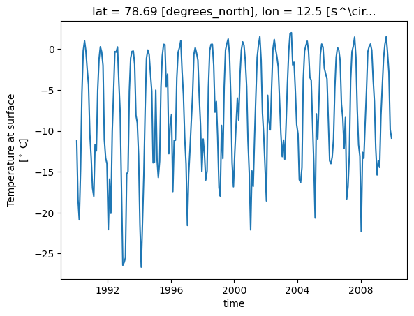
6. The easiest interpolation: select with ‘nearest’ neighboor

Example: let’s select Zeppelin station: 78.906661, 11.889203

lat_zep = 78.90
lon_zep = 11.89

dss['T_C'].sel(lon=lon_zep, lat=lat_zep, method='nearest').plot()

[<matplotlib.lines.Line2D at 0x7f7eaa505610>]

7. Super quick averaging etc with xarray

da_so4 = dss['mmrso4']
da_so4

<xarray.DataArray 'mmrso4' (member_id: 1, dcpp_init_year: 1, time: 240,
                            lev: 32, lat: 192, lon: 288)> Size: 2GB
dask.array<getitem, shape=(1, 1, 240, 32, 192, 288), dtype=float32, chunksize=(1, 1, 10, 32, 192, 288), chunktype=numpy.ndarray>
Coordinates:
  * member_id       (member_id) object 8B 'r1i1p1f1'
  * dcpp_init_year  (dcpp_init_year) object 8B None
  * time            (time) datetime64[ns] 2kB 1990-01-15T12:00:00 ... 2009-12...
  * lev             (lev) float64 256B -3.643 -7.595 -14.36 ... -976.3 -992.6
  * lat             (lat) float64 2kB -90.0 -89.06 -88.12 ... 88.12 89.06 90.0
  * lon             (lon) float64 2kB -180.0 -178.8 -177.5 ... 176.2 177.5 178.8
Attributes: (12/19)
    cell_measures:  area: areacella
    cell_methods:   area: time: mean
    comment:        Dry mass of sulfate (SO4) in aerosol particles as a fract...
    description:    Dry mass of sulfate (SO4) in aerosol particles as a fract...
    frequency:      mon
    id:             mmrso4
    ...             ...
    time_label:     time-mean
    time_title:     Temporal mean
    title:          Aerosol Sulfate Mass Mixing Ratio
    type:           real
    units:          kg kg-1
    variable_id:    mmrso4

xarray.DataArray

'mmrso4'

• member_id: 1
• dcpp_init_year: 1
• time: 240
• lev: 32
• lat: 192
• lon: 288

• dask.array<chunksize=(1, 1, 10, 32, 192, 288), meta=np.ndarray>

  Array Chunk Bytes 1.58 GiB 67.50 MiB Shape (1, 1, 240, 32, 192, 288) (1, 1, 10, 32, 192, 288) Dask graph 24 chunks in 5 graph layers Data type float32 numpy.ndarray

• Coordinates: (6)
  • member_id
    (member_id)
    object
    'r1i1p1f1'

    array(['r1i1p1f1'], dtype=object)

  • dcpp_init_year
    (dcpp_init_year)
    object
    None

    array([None], dtype=object)

  • time
    (time)
    datetime64[ns]
    1990-01-15T12:00:00 ... 2009-12-...

    array(['1990-01-15T12:00:00.000000000', '1990-02-14T00:00:00.000000000',
           '1990-03-15T12:00:00.000000000', ..., '2009-10-15T12:00:00.000000000',
           '2009-11-15T00:00:00.000000000', '2009-12-15T12:00:00.000000000'],
          shape=(240,), dtype='datetime64[ns]')

  • lev
    (lev)
    float64
    -3.643 -7.595 ... -976.3 -992.6

    axis :

    Z

    bounds :

    lev_bnds

    positive :

    up

    standard_name :

    alevel

    title :

    atmospheric model level

    type :

    double

    units :

    hPa

    array([  -3.643466,   -7.59482 ,  -14.356632,  -24.61222 ,  -35.92325 ,
            -43.19375 ,  -51.677499,  -61.520498,  -73.750958,  -87.82123 ,
           -103.317127, -121.547241, -142.994039, -168.22508 , -197.908087,
           -232.828619, -273.910817, -322.241902, -379.100904, -445.992574,
           -524.687175, -609.778695, -691.38943 , -763.404481, -820.858369,
           -859.534767, -887.020249, -912.644547, -936.198398, -957.48548 ,
           -976.325407, -992.556095])

  • lat
    (lat)
    float64
    -90.0 -89.06 -88.12 ... 89.06 90.0

    axis :

    Y

    bounds :

    lat_bnds

    standard_name :

    latitude

    title :

    Latitude

    type :

    double

    units :

    degrees_north

    valid_max :

    90.0

    valid_min :

    -90.0

    array([-90.      , -89.057592, -88.115183, -87.172775, -86.230366, -85.287958,
           -84.34555 , -83.403141, -82.460733, -81.518325, -80.575916, -79.633508,
           -78.691099, -77.748691, -76.806283, -75.863874, -74.921466, -73.979058,
           -73.036649, -72.094241, -71.151832, -70.209424, -69.267016, -68.324607,
           -67.382199, -66.439791, -65.497382, -64.554974, -63.612565, -62.670157,
           -61.727749, -60.78534 , -59.842932, -58.900524, -57.958115, -57.015707,
           -56.073298, -55.13089 , -54.188482, -53.246073, -52.303665, -51.361257,
           -50.418848, -49.47644 , -48.534031, -47.591623, -46.649215, -45.706806,
           -44.764398, -43.82199 , -42.879581, -41.937173, -40.994764, -40.052356,
           -39.109948, -38.167539, -37.225131, -36.282723, -35.340314, -34.397906,
           -33.455497, -32.513089, -31.570681, -30.628272, -29.685864, -28.743455,
           -27.801047, -26.858639, -25.91623 , -24.973822, -24.031414, -23.089005,
           -22.146597, -21.204188, -20.26178 , -19.319372, -18.376963, -17.434555,
           -16.492147, -15.549738, -14.60733 , -13.664921, -12.722513, -11.780105,
           -10.837696,  -9.895288,  -8.95288 ,  -8.010471,  -7.068063,  -6.125654,
            -5.183246,  -4.240838,  -3.298429,  -2.356021,  -1.413613,  -0.471204,
             0.471204,   1.413613,   2.356021,   3.298429,   4.240838,   5.183246,
             6.125654,   7.068063,   8.010471,   8.95288 ,   9.895288,  10.837696,
            11.780105,  12.722513,  13.664921,  14.60733 ,  15.549738,  16.492147,
            17.434555,  18.376963,  19.319372,  20.26178 ,  21.204188,  22.146597,
            23.089005,  24.031414,  24.973822,  25.91623 ,  26.858639,  27.801047,
            28.743455,  29.685864,  30.628272,  31.570681,  32.513089,  33.455497,
            34.397906,  35.340314,  36.282723,  37.225131,  38.167539,  39.109948,
            40.052356,  40.994764,  41.937173,  42.879581,  43.82199 ,  44.764398,
            45.706806,  46.649215,  47.591623,  48.534031,  49.47644 ,  50.418848,
            51.361257,  52.303665,  53.246073,  54.188482,  55.13089 ,  56.073298,
            57.015707,  57.958115,  58.900524,  59.842932,  60.78534 ,  61.727749,
            62.670157,  63.612565,  64.554974,  65.497382,  66.439791,  67.382199,
            68.324607,  69.267016,  70.209424,  71.151832,  72.094241,  73.036649,
            73.979058,  74.921466,  75.863874,  76.806283,  77.748691,  78.691099,
            79.633508,  80.575916,  81.518325,  82.460733,  83.403141,  84.34555 ,
            85.287958,  86.230366,  87.172775,  88.115183,  89.057592,  90.      ])

  • lon
    (lon)
    float64
    -180.0 -178.8 ... 177.5 178.8

    axis :

    X

    bounds :

    lon_bnds

    standard_name :

    longitude

    title :

    Longitude

    type :

    double

    units :

    $^\circ$ East

    valid_max :

    360.0

    valid_min :

    0.0

    array([-180.  , -178.75, -177.5 , ...,  176.25,  177.5 ,  178.75], shape=(288,))

• Attributes: (19)

  cell_measures :

  area: areacella

  cell_methods :

  area: time: mean

  comment :

  Dry mass of sulfate (SO4) in aerosol particles as a fraction of air mass.

  description :

  Dry mass of sulfate (SO4) in aerosol particles as a fraction of air mass.

  frequency :

  mon

  id :

  mmrso4

  long_name :

  Aerosol Sulfate Mass Mixing Ratio

  mipTable :

  AERmon

  out_name :

  mmrso4

  prov :

  AERmon ((isd.003))

  realm :

  aerosol

  standard_name :

  mass_fraction_of_sulfate_dry_aerosol_particles_in_air

  time :

  time

  time_label :

  time-mean

  time_title :

  Temporal mean

  title :

  Aerosol Sulfate Mass Mixing Ratio

  type :

  real

  units :

  kg kg-1

  variable_id :

  mmrso4

Mean:

da_so4_lmean = da_so4.mean(['time','lon'], keep_attrs=True) #.plot()#ylim=[1000,100], yscale='log')

da_so4_lmean

<xarray.DataArray 'mmrso4' (member_id: 1, dcpp_init_year: 1, lev: 32, lat: 192)> Size: 25kB
dask.array<mean_agg-aggregate, shape=(1, 1, 32, 192), dtype=float32, chunksize=(1, 1, 32, 192), chunktype=numpy.ndarray>
Coordinates:
  * member_id       (member_id) object 8B 'r1i1p1f1'
  * dcpp_init_year  (dcpp_init_year) object 8B None
  * lev             (lev) float64 256B -3.643 -7.595 -14.36 ... -976.3 -992.6
  * lat             (lat) float64 2kB -90.0 -89.06 -88.12 ... 88.12 89.06 90.0
Attributes: (12/19)
    cell_measures:  area: areacella
    cell_methods:   area: time: mean
    comment:        Dry mass of sulfate (SO4) in aerosol particles as a fract...
    description:    Dry mass of sulfate (SO4) in aerosol particles as a fract...
    frequency:      mon
    id:             mmrso4
    ...             ...
    time_label:     time-mean
    time_title:     Temporal mean
    title:          Aerosol Sulfate Mass Mixing Ratio
    type:           real
    units:          kg kg-1
    variable_id:    mmrso4

xarray.DataArray

'mmrso4'

• member_id: 1
• dcpp_init_year: 1
• lev: 32
• lat: 192

• dask.array<chunksize=(1, 1, 32, 192), meta=np.ndarray>

  Array Chunk Bytes 24.00 kiB 24.00 kiB Shape (1, 1, 32, 192) (1, 1, 32, 192) Dask graph 1 chunks in 11 graph layers Data type float32 numpy.ndarray

• Coordinates: (4)
  • member_id
    (member_id)
    object
    'r1i1p1f1'

    array(['r1i1p1f1'], dtype=object)

  • dcpp_init_year
    (dcpp_init_year)
    object
    None

    array([None], dtype=object)

  • lev
    (lev)
    float64
    -3.643 -7.595 ... -976.3 -992.6

    axis :

    Z

    bounds :

    lev_bnds

    positive :

    up

    standard_name :

    alevel

    title :

    atmospheric model level

    type :

    double

    units :

    hPa

    array([  -3.643466,   -7.59482 ,  -14.356632,  -24.61222 ,  -35.92325 ,
            -43.19375 ,  -51.677499,  -61.520498,  -73.750958,  -87.82123 ,
           -103.317127, -121.547241, -142.994039, -168.22508 , -197.908087,
           -232.828619, -273.910817, -322.241902, -379.100904, -445.992574,
           -524.687175, -609.778695, -691.38943 , -763.404481, -820.858369,
           -859.534767, -887.020249, -912.644547, -936.198398, -957.48548 ,
           -976.325407, -992.556095])

  • lat
    (lat)
    float64
    -90.0 -89.06 -88.12 ... 89.06 90.0

    axis :

    Y

    bounds :

    lat_bnds

    standard_name :

    latitude

    title :

    Latitude

    type :

    double

    units :

    degrees_north

    valid_max :

    90.0

    valid_min :

    -90.0

    array([-90.      , -89.057592, -88.115183, -87.172775, -86.230366, -85.287958,
           -84.34555 , -83.403141, -82.460733, -81.518325, -80.575916, -79.633508,
           -78.691099, -77.748691, -76.806283, -75.863874, -74.921466, -73.979058,
           -73.036649, -72.094241, -71.151832, -70.209424, -69.267016, -68.324607,
           -67.382199, -66.439791, -65.497382, -64.554974, -63.612565, -62.670157,
           -61.727749, -60.78534 , -59.842932, -58.900524, -57.958115, -57.015707,
           -56.073298, -55.13089 , -54.188482, -53.246073, -52.303665, -51.361257,
           -50.418848, -49.47644 , -48.534031, -47.591623, -46.649215, -45.706806,
           -44.764398, -43.82199 , -42.879581, -41.937173, -40.994764, -40.052356,
           -39.109948, -38.167539, -37.225131, -36.282723, -35.340314, -34.397906,
           -33.455497, -32.513089, -31.570681, -30.628272, -29.685864, -28.743455,
           -27.801047, -26.858639, -25.91623 , -24.973822, -24.031414, -23.089005,
           -22.146597, -21.204188, -20.26178 , -19.319372, -18.376963, -17.434555,
           -16.492147, -15.549738, -14.60733 , -13.664921, -12.722513, -11.780105,
           -10.837696,  -9.895288,  -8.95288 ,  -8.010471,  -7.068063,  -6.125654,
            -5.183246,  -4.240838,  -3.298429,  -2.356021,  -1.413613,  -0.471204,
             0.471204,   1.413613,   2.356021,   3.298429,   4.240838,   5.183246,
             6.125654,   7.068063,   8.010471,   8.95288 ,   9.895288,  10.837696,
            11.780105,  12.722513,  13.664921,  14.60733 ,  15.549738,  16.492147,
            17.434555,  18.376963,  19.319372,  20.26178 ,  21.204188,  22.146597,
            23.089005,  24.031414,  24.973822,  25.91623 ,  26.858639,  27.801047,
            28.743455,  29.685864,  30.628272,  31.570681,  32.513089,  33.455497,
            34.397906,  35.340314,  36.282723,  37.225131,  38.167539,  39.109948,
            40.052356,  40.994764,  41.937173,  42.879581,  43.82199 ,  44.764398,
            45.706806,  46.649215,  47.591623,  48.534031,  49.47644 ,  50.418848,
            51.361257,  52.303665,  53.246073,  54.188482,  55.13089 ,  56.073298,
            57.015707,  57.958115,  58.900524,  59.842932,  60.78534 ,  61.727749,
            62.670157,  63.612565,  64.554974,  65.497382,  66.439791,  67.382199,
            68.324607,  69.267016,  70.209424,  71.151832,  72.094241,  73.036649,
            73.979058,  74.921466,  75.863874,  76.806283,  77.748691,  78.691099,
            79.633508,  80.575916,  81.518325,  82.460733,  83.403141,  84.34555 ,
            85.287958,  86.230366,  87.172775,  88.115183,  89.057592,  90.      ])

• Attributes: (19)

  cell_measures :

  area: areacella

  cell_methods :

  area: time: mean

  comment :

  Dry mass of sulfate (SO4) in aerosol particles as a fraction of air mass.

  description :

  Dry mass of sulfate (SO4) in aerosol particles as a fraction of air mass.

  frequency :

  mon

  id :

  mmrso4

  long_name :

  Aerosol Sulfate Mass Mixing Ratio

  mipTable :

  AERmon

  out_name :

  mmrso4

  prov :

  AERmon ((isd.003))

  realm :

  aerosol

  standard_name :

  mass_fraction_of_sulfate_dry_aerosol_particles_in_air

  time :

  time

  time_label :

  time-mean

  time_title :

  Temporal mean

  title :

  Aerosol Sulfate Mass Mixing Ratio

  type :

  real

  units :

  kg kg-1

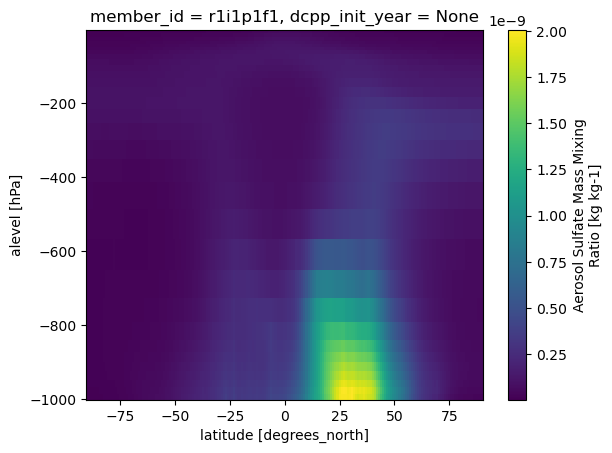
  variable_id :

  mmrso4

8. Plotting with xarray

• Notice it’s slow now, why?

da_so4_lmean.plot()

<matplotlib.collections.QuadMesh at 0x7f7df23e0a40>

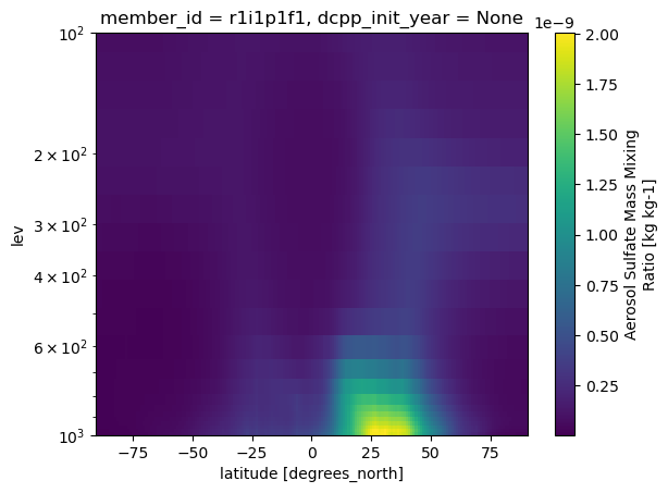
da_so4_lmean['lev'] = np.abs(da_so4_lmean['lev'].values)

da_so4_lmean.plot(
    ylim=[1000,100], 
    yscale='log'
)

<matplotlib.collections.QuadMesh at 0x7f7df0e74e30>

Standard deviation

dss['T_C'].std(['time']).plot()

<matplotlib.collections.QuadMesh at 0x7f7df046e8a0>

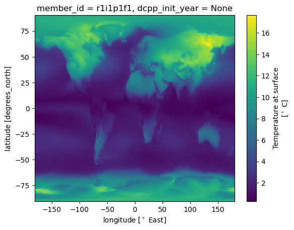
Temperature change much stronger over land than ocean and higher at high latitudes…

9. Mask data and groupby: pick out seasons

month = ds['time.month']

month

<xarray.DataArray 'month' (time: 1980)> Size: 16kB
array([ 1,  2,  3, ..., 10, 11, 12], shape=(1980,))
Coordinates:
  * time     (time) object 16kB 1850-01-15 12:00:00 ... 2014-12-15 12:00:00

xarray.DataArray

'month'

• time: 1980

• 1 2 3 4 5 6 7 8 9 10 11 12 1 2 3 ... 11 12 1 2 3 4 5 6 7 8 9 10 11 12

  array([ 1,  2,  3, ..., 10, 11, 12], shape=(1980,))

• Coordinates: (1)
  • time
    (time)
    object
    1850-01-15 12:00:00 ... 2014-12-...

    axis :

    T

    bounds :

    time_bnds

    standard_name :

    time

    title :

    time

    type :

    double

    array([cftime.DatetimeNoLeap(1850, 1, 15, 12, 0, 0, 0, has_year_zero=True),
           cftime.DatetimeNoLeap(1850, 2, 14, 0, 0, 0, 0, has_year_zero=True),
           cftime.DatetimeNoLeap(1850, 3, 15, 12, 0, 0, 0, has_year_zero=True),
           ...,
           cftime.DatetimeNoLeap(2014, 10, 15, 12, 0, 0, 0, has_year_zero=True),
           cftime.DatetimeNoLeap(2014, 11, 15, 0, 0, 0, 0, has_year_zero=True),
           cftime.DatetimeNoLeap(2014, 12, 15, 12, 0, 0, 0, has_year_zero=True)],
          shape=(1980,), dtype=object)

dss_JA = (dss
    .where(month.isin([7,8]))
    .mean('time')
         )

dss_JA

<xarray.Dataset> Size: 8MB
Dimensions:         (member_id: 1, dcpp_init_year: 1, lat: 192, lon: 288,
                     lev: 32, nbnd: 2)
Coordinates:
  * member_id       (member_id) object 8B 'r1i1p1f1'
  * dcpp_init_year  (dcpp_init_year) object 8B None
  * lat             (lat) float64 2kB -90.0 -89.06 -88.12 ... 88.12 89.06 90.0
  * lon             (lon) float64 2kB -180.0 -178.8 -177.5 ... 176.2 177.5 178.8
  * lev             (lev) float64 256B -3.643 -7.595 -14.36 ... -976.3 -992.6
    a_bnds          (lev, nbnd) float64 512B dask.array<chunksize=(32, 2), meta=np.ndarray>
    b_bnds          (lev, nbnd) float64 512B dask.array<chunksize=(32, 2), meta=np.ndarray>
    lev_bnds        (lev, nbnd) float64 512B dask.array<chunksize=(32, 2), meta=np.ndarray>
Dimensions without coordinates: nbnd
Data variables:
    areacella       (member_id, dcpp_init_year, lat, lon) float32 221kB dask.array<chunksize=(1, 1, 192, 288), meta=np.ndarray>
    a               (lev) float64 256B dask.array<chunksize=(32,), meta=np.ndarray>
    b               (lev) float64 256B dask.array<chunksize=(32,), meta=np.ndarray>
    mmrso4          (member_id, dcpp_init_year, lev, lat, lon) float32 7MB dask.array<chunksize=(1, 1, 32, 192, 288), meta=np.ndarray>
    p0              float32 4B nan
    ps              (lat, lon) float32 221kB dask.array<chunksize=(192, 288), meta=np.ndarray>
    hurs            (member_id, dcpp_init_year, lat, lon) float32 221kB dask.array<chunksize=(1, 1, 192, 288), meta=np.ndarray>
    tas             (member_id, dcpp_init_year, lat, lon) float32 221kB dask.array<chunksize=(1, 1, 192, 288), meta=np.ndarray>
    T_C             (member_id, dcpp_init_year, lat, lon) float32 221kB dask.array<chunksize=(1, 1, 192, 288), meta=np.ndarray>
Attributes: (12/58)
    Conventions:                      CF-1.7 CMIP-6.2
    activity_id:                      CMIP
    branch_method:                    standard
    branch_time_in_child:             674885.0
    branch_time_in_parent:            219000.0
    case_id:                          15
    ...                               ...
    intake_esm_attrs:variable_id:     areacella
    intake_esm_attrs:grid_label:      gn
    intake_esm_attrs:zstore:          gs://cmip6/CMIP6/CMIP/NCAR/CESM2/histor...
    intake_esm_attrs:version:         20190308
    intake_esm_attrs:_data_format_:   zarr
    intake_esm_dataset_key:           CMIP.historical.CESM2.fx.gn

xarray.Dataset

• Dimensions:
  • member_id: 1
  • dcpp_init_year: 1
  • lat: 192
  • lon: 288
  • lev: 32
  • nbnd: 2
• Coordinates: (8)
  • member_id
    (member_id)
    object
    'r1i1p1f1'

    array(['r1i1p1f1'], dtype=object)

  • dcpp_init_year
    (dcpp_init_year)
    object
    None

    array([None], dtype=object)

  • lat
    (lat)
    float64
    -90.0 -89.06 -88.12 ... 89.06 90.0

    axis :

    Y

    bounds :

    lat_bnds

    standard_name :

    latitude

    title :

    Latitude

    type :

    double

    units :

    degrees_north

    valid_max :

    90.0

    valid_min :

    -90.0

    array([-90.      , -89.057592, -88.115183, -87.172775, -86.230366, -85.287958,
           -84.34555 , -83.403141, -82.460733, -81.518325, -80.575916, -79.633508,
           -78.691099, -77.748691, -76.806283, -75.863874, -74.921466, -73.979058,
           -73.036649, -72.094241, -71.151832, -70.209424, -69.267016, -68.324607,
           -67.382199, -66.439791, -65.497382, -64.554974, -63.612565, -62.670157,
           -61.727749, -60.78534 , -59.842932, -58.900524, -57.958115, -57.015707,
           -56.073298, -55.13089 , -54.188482, -53.246073, -52.303665, -51.361257,
           -50.418848, -49.47644 , -48.534031, -47.591623, -46.649215, -45.706806,
           -44.764398, -43.82199 , -42.879581, -41.937173, -40.994764, -40.052356,
           -39.109948, -38.167539, -37.225131, -36.282723, -35.340314, -34.397906,
           -33.455497, -32.513089, -31.570681, -30.628272, -29.685864, -28.743455,
           -27.801047, -26.858639, -25.91623 , -24.973822, -24.031414, -23.089005,
           -22.146597, -21.204188, -20.26178 , -19.319372, -18.376963, -17.434555,
           -16.492147, -15.549738, -14.60733 , -13.664921, -12.722513, -11.780105,
           -10.837696,  -9.895288,  -8.95288 ,  -8.010471,  -7.068063,  -6.125654,
            -5.183246,  -4.240838,  -3.298429,  -2.356021,  -1.413613,  -0.471204,
             0.471204,   1.413613,   2.356021,   3.298429,   4.240838,   5.183246,
             6.125654,   7.068063,   8.010471,   8.95288 ,   9.895288,  10.837696,
            11.780105,  12.722513,  13.664921,  14.60733 ,  15.549738,  16.492147,
            17.434555,  18.376963,  19.319372,  20.26178 ,  21.204188,  22.146597,
            23.089005,  24.031414,  24.973822,  25.91623 ,  26.858639,  27.801047,
            28.743455,  29.685864,  30.628272,  31.570681,  32.513089,  33.455497,
            34.397906,  35.340314,  36.282723,  37.225131,  38.167539,  39.109948,
            40.052356,  40.994764,  41.937173,  42.879581,  43.82199 ,  44.764398,
            45.706806,  46.649215,  47.591623,  48.534031,  49.47644 ,  50.418848,
            51.361257,  52.303665,  53.246073,  54.188482,  55.13089 ,  56.073298,
            57.015707,  57.958115,  58.900524,  59.842932,  60.78534 ,  61.727749,
            62.670157,  63.612565,  64.554974,  65.497382,  66.439791,  67.382199,
            68.324607,  69.267016,  70.209424,  71.151832,  72.094241,  73.036649,
            73.979058,  74.921466,  75.863874,  76.806283,  77.748691,  78.691099,
            79.633508,  80.575916,  81.518325,  82.460733,  83.403141,  84.34555 ,
            85.287958,  86.230366,  87.172775,  88.115183,  89.057592,  90.      ])

  • lon
    (lon)
    float64
    -180.0 -178.8 ... 177.5 178.8

    axis :

    X

    bounds :

    lon_bnds

    standard_name :

    longitude

    title :

    Longitude

    type :

    double

    units :

    $^\circ$ East

    valid_max :

    360.0

    valid_min :

    0.0

    array([-180.  , -178.75, -177.5 , ...,  176.25,  177.5 ,  178.75], shape=(288,))

  • lev
    (lev)
    float64
    -3.643 -7.595 ... -976.3 -992.6

    axis :

    Z

    bounds :

    lev_bnds

    positive :

    up

    standard_name :

    alevel

    title :

    atmospheric model level

    type :

    double

    units :

    hPa

    array([  -3.643466,   -7.59482 ,  -14.356632,  -24.61222 ,  -35.92325 ,
            -43.19375 ,  -51.677499,  -61.520498,  -73.750958,  -87.82123 ,
           -103.317127, -121.547241, -142.994039, -168.22508 , -197.908087,
           -232.828619, -273.910817, -322.241902, -379.100904, -445.992574,
           -524.687175, -609.778695, -691.38943 , -763.404481, -820.858369,
           -859.534767, -887.020249, -912.644547, -936.198398, -957.48548 ,
           -976.325407, -992.556095])

  • a_bnds
    (lev, nbnd)
    float64
    dask.array<chunksize=(32, 2), meta=np.ndarray>

    long_name :

    vertical coordinate formula term: a(k+1/2)

    Array Chunk Bytes 512 B 512 B Shape (32, 2) (32, 2) Dask graph 1 chunks in 2 graph layers Data type float64 numpy.ndarray

  • b_bnds
    (lev, nbnd)
    float64
    dask.array<chunksize=(32, 2), meta=np.ndarray>

    long_name :

    vertical coordinate formula term: b(k+1/2)

    Array Chunk Bytes 512 B 512 B Shape (32, 2) (32, 2) Dask graph 1 chunks in 2 graph layers Data type float64 numpy.ndarray

  • lev_bnds
    (lev, nbnd)
    float64
    dask.array<chunksize=(32, 2), meta=np.ndarray>

    formula :

    p = a*p0 + b*ps

    formula_terms :

    p0: p0 a: a_bnds b: b_bnds ps: ps

    standard_name :

    atmosphere_hybrid_sigma_pressure_coordinate

    units :

    hPa

    Array Chunk Bytes 512 B 512 B Shape (32, 2) (32, 2) Dask graph 1 chunks in 2 graph layers Data type float64 numpy.ndarray

• Data variables: (9)
  • areacella
    (member_id, dcpp_init_year, lat, lon)
    float32
    dask.array<chunksize=(1, 1, 192, 288), meta=np.ndarray>

    cell_methods :

    area: sum

    comment :

    Cell areas for any grid used to report atmospheric variables and any other variable using that grid (e.g., soil moisture content). These cell areas should be defined to enable exact calculation of global integrals (e.g., of vertical fluxes of energy at the surface and top of the atmosphere).

    description :

    Cell areas for any grid used to report atmospheric variables and any other variable using that grid (e.g., soil moisture content). These cell areas should be defined to enable exact calculation of global integrals (e.g., of vertical fluxes of energy at the surface and top of the atmosphere).

    frequency :

    fx

    id :

    areacella

    long_name :

    Grid-Cell Area for Atmospheric Grid Variables

    mipTable :

    fx

    out_name :

    areacella

    prov :

    fx ((isd.003))

    realm :

    atmos land

    standard_name :

    cell_area

    time_label :

    None

    time_title :

    No temporal dimensions ... fixed field

    title :

    Grid-Cell Area for Atmospheric Grid Variables

    type :

    real

    units :

    m2

    variable_id :

    areacella

    Array Chunk Bytes 216.00 kiB 216.00 kiB Shape (1, 1, 192, 288) (1, 1, 192, 288) Dask graph 1 chunks in 9 graph layers Data type float32 numpy.ndarray

  • a
    (lev)
    float64
    dask.array<chunksize=(32,), meta=np.ndarray>

    bounds :

    a_bnds

    long_name :

    vertical coordinate formula term: a(k)

    Array Chunk Bytes 256 B 256 B Shape (32,) (32,) Dask graph 1 chunks in 7 graph layers Data type float64 numpy.ndarray

  • b
    (lev)
    float64
    dask.array<chunksize=(32,), meta=np.ndarray>

    bounds :

    b_bnds

    long_name :

    vertical coordinate formula term: b(k)

    Array Chunk Bytes 256 B 256 B Shape (32,) (32,) Dask graph 1 chunks in 7 graph layers Data type float64 numpy.ndarray

  • mmrso4
    (member_id, dcpp_init_year, lev, lat, lon)
    float32
    dask.array<chunksize=(1, 1, 32, 192, 288), meta=np.ndarray>

    cell_measures :

    area: areacella

    cell_methods :

    area: time: mean

    comment :

    Dry mass of sulfate (SO4) in aerosol particles as a fraction of air mass.

    description :

    Dry mass of sulfate (SO4) in aerosol particles as a fraction of air mass.

    frequency :

    mon

    id :

    mmrso4

    long_name :

    Aerosol Sulfate Mass Mixing Ratio

    mipTable :

    AERmon

    out_name :

    mmrso4

    prov :

    AERmon ((isd.003))

    realm :

    aerosol

    standard_name :

    mass_fraction_of_sulfate_dry_aerosol_particles_in_air

    time :

    time

    time_label :

    time-mean

    time_title :

    Temporal mean

    title :

    Aerosol Sulfate Mass Mixing Ratio

    type :

    real

    units :

    kg kg-1

    variable_id :

    mmrso4

    Array Chunk Bytes 6.75 MiB 6.75 MiB Shape (1, 1, 32, 192, 288) (1, 1, 32, 192, 288) Dask graph 1 chunks in 10 graph layers Data type float32 numpy.ndarray

  • p0
    ()
    float32
    nan

    long_name :

    vertical coordinate formula term: reference pressure

    units :

    Pa

    array(nan, dtype=float32)

  • ps
    (lat, lon)
    float32
    dask.array<chunksize=(192, 288), meta=np.ndarray>

    long_name :

    surface_air_pressure

    units :

    Pa

    Array Chunk Bytes 216.00 kiB 216.00 kiB Shape (192, 288) (192, 288) Dask graph 1 chunks in 9 graph layers Data type float32 numpy.ndarray

  • hurs
    (member_id, dcpp_init_year, lat, lon)
    float32
    dask.array<chunksize=(1, 1, 192, 288), meta=np.ndarray>

    cell_measures :

    area: areacella

    cell_methods :

    area: time: mean

    comment :

    This is the relative humidity with respect to liquid water for T> 0 C, and with respect to ice for T<0 C.

    description :

    This is the relative humidity with respect to liquid water for T> 0 C, and with respect to ice for T<0 C.

    frequency :

    mon

    id :

    hurs

    long_name :

    Near-Surface Relative Humidity

    mipTable :

    Amon

    out_name :

    hurs

    prov :

    Amon ((isd.003))

    realm :

    atmos

    standard_name :

    relative_humidity

    time :

    time

    time_label :

    time-mean

    time_title :

    Temporal mean

    title :

    Near-Surface Relative Humidity

    type :

    real

    units :

    %

    variable_id :

    hurs

    Array Chunk Bytes 216.00 kiB 216.00 kiB Shape (1, 1, 192, 288) (1, 1, 192, 288) Dask graph 1 chunks in 10 graph layers Data type float32 numpy.ndarray

  • tas
    (member_id, dcpp_init_year, lat, lon)
    float32
    dask.array<chunksize=(1, 1, 192, 288), meta=np.ndarray>

    cell_measures :

    area: areacella

    cell_methods :

    area: time: mean

    comment :

    near-surface (usually, 2 meter) air temperature

    description :

    near-surface (usually, 2 meter) air temperature

    frequency :

    mon

    id :

    tas

    long_name :

    Near-Surface Air Temperature

    mipTable :

    Amon

    out_name :

    tas

    prov :

    Amon ((isd.003))

    realm :

    atmos

    standard_name :

    air_temperature

    time :

    time

    time_label :

    time-mean

    time_title :

    Temporal mean

    title :

    Near-Surface Air Temperature

    type :

    real

    units :

    K

    variable_id :

    tas

    Array Chunk Bytes 216.00 kiB 216.00 kiB Shape (1, 1, 192, 288) (1, 1, 192, 288) Dask graph 1 chunks in 10 graph layers Data type float32 numpy.ndarray

  • T_C
    (member_id, dcpp_init_year, lat, lon)
    float32
    dask.array<chunksize=(1, 1, 192, 288), meta=np.ndarray>

    cell_measures :

    area: areacella

    cell_methods :

    area: time: mean

    comment :

    near-surface (usually, 2 meter) air temperature

    description :

    near-surface (usually, 2 meter) air temperature

    frequency :

    mon

    id :

    tas

    long_name :

    Temperature at surface

    mipTable :

    Amon

    out_name :

    tas

    prov :

    Amon ((isd.003))

    realm :

    atmos

    standard_name :

    air_temperature

    time :

    time

    time_label :

    time-mean

    time_title :

    Temporal mean

    title :

    Near-Surface Air Temperature

    type :

    real

    units :

    $^\circ$ C

    variable_id :

    tas

    Array Chunk Bytes 216.00 kiB 216.00 kiB Shape (1, 1, 192, 288) (1, 1, 192, 288) Dask graph 1 chunks in 11 graph layers Data type float32 numpy.ndarray

• Attributes: (58)

  Conventions :

  CF-1.7 CMIP-6.2

  activity_id :

  CMIP

  branch_method :

  standard

  branch_time_in_child :

  674885.0

  branch_time_in_parent :

  219000.0

  case_id :

  15

  cesm_casename :

  b.e21.BHIST.f09_g17.CMIP6-historical.001

  contact :

  cesm_cmip6@ucar.edu

  creation_date :

  2019-01-16T21:43:39Z

  data_specs_version :

  01.00.29

  experiment :

  all-forcing simulation of the recent past

  experiment_id :

  historical

  forcing_index :

  1

  frequency :

  fx

  further_info_url :

  https://furtherinfo.es-doc.org/CMIP6.NCAR.CESM2.historical.none.r1i1p1f1

  grid :

  native 0.9x1.25 finite volume grid (192x288 latxlon)

  grid_label :

  gn

  initialization_index :

  1

  institution :

  National Center for Atmospheric Research, Climate and Global Dynamics Laboratory, 1850 Table Mesa Drive, Boulder, CO 80305, USA

  institution_id :

  NCAR

  license :

  CMIP6 model data produced by <The National Center for Atmospheric Research> is licensed under a Creative Commons Attribution-[]ShareAlike 4.0 International License (https://creativecommons.org/licenses/). Consult https://pcmdi.llnl.gov/CMIP6/TermsOfUse for terms of use governing CMIP6 output, including citation requirements and proper acknowledgment. Further information about this data, including some limitations, can be found via the further_info_url (recorded as a global attribute in this file)[]. The data producers and data providers make no warranty, either express or implied, including, but not limited to, warranties of merchantability and fitness for a particular purpose. All liabilities arising from the supply of the information (including any liability arising in negligence) are excluded to the fullest extent permitted by law.

  mip_era :

  CMIP6

  model_doi_url :

  https://doi.org/10.5065/D67H1H0V

  nominal_resolution :

  100 km

  parent_activity_id :

  CMIP

  parent_experiment_id :

  piControl

  parent_mip_era :

  CMIP6

  parent_source_id :

  CESM2

  parent_time_units :

  days since 0001-01-01 00:00:00

  parent_variant_label :

  r1i1p1f1

  physics_index :

  1

  product :

  model-output

  realization_index :

  1

  realm :

  atmos land

  source :

  CESM2 (2017): atmosphere: CAM6 (0.9x1.25 finite volume grid; 288 x 192 longitude/latitude; 32 levels; top level 2.25 mb); ocean: POP2 (320x384 longitude/latitude; 60 levels; top grid cell 0-10 m); sea_ice: CICE5.1 (same grid as ocean); land: CLM5 0.9x1.25 finite volume grid; 288 x 192 longitude/latitude; 32 levels; top level 2.25 mb); aerosol: MAM4 (0.9x1.25 finite volume grid; 288 x 192 longitude/latitude; 32 levels; top level 2.25 mb); atmoschem: MAM4 (0.9x1.25 finite volume grid; 288 x 192 longitude/latitude; 32 levels; top level 2.25 mb); landIce: CISM2.1; ocnBgchem: MARBL (320x384 longitude/latitude; 60 levels; top grid cell 0-10 m)

  source_id :

  CESM2

  source_type :

  AOGCM BGC

  sub_experiment :

  none

  sub_experiment_id :

  none

  table_id :

  fx

  tracking_id :

  hdl:21.14100/75033260-7bd2-46b9-9d98-3456f176d588

  variable_id :

  areacella

  variant_info :

  CMIP6 20th century experiments (1850-2014) with CAM6, interactive land (CLM5), coupled ocean (POP2) with biogeochemistry (MARBL), interactive sea ice (CICE5.1), and non-evolving land ice (CISM2.1)

  variant_label :

  r1i1p1f1

  status :

  2019-10-25;created;by nhn2@columbia.edu

  intake_esm_vars :

  ['areacella']

  intake_esm_attrs:activity_id :

  CMIP

  intake_esm_attrs:institution_id :

  NCAR

  intake_esm_attrs:source_id :

  CESM2

  intake_esm_attrs:experiment_id :

  historical

  intake_esm_attrs:member_id :

  r1i1p1f1

  intake_esm_attrs:table_id :

  fx

  intake_esm_attrs:variable_id :

  areacella

  intake_esm_attrs:grid_label :

  gn

  intake_esm_attrs:zstore :

  gs://cmip6/CMIP6/CMIP/NCAR/CESM2/historical/r1i1p1f1/fx/areacella/gn/v20190308/

  intake_esm_attrs:version :

  20190308

  intake_esm_attrs:_data_format_ :

  zarr

  intake_esm_dataset_key :

  CMIP.historical.CESM2.fx.gn

dss_season = (dss
    .groupby('time.season')
    .mean(keep_attrs=True)
             )

dss_season

<xarray.Dataset> Size: 33MB
Dimensions:         (season: 4, member_id: 1, dcpp_init_year: 1, lev: 32,
                     lat: 192, lon: 288, nbnd: 2)
Coordinates:
  * season          (season) object 32B 'DJF' 'JJA' 'MAM' 'SON'
  * member_id       (member_id) object 8B 'r1i1p1f1'
  * dcpp_init_year  (dcpp_init_year) object 8B None
  * lev             (lev) float64 256B -3.643 -7.595 -14.36 ... -976.3 -992.6
  * lat             (lat) float64 2kB -90.0 -89.06 -88.12 ... 88.12 89.06 90.0
  * lon             (lon) float64 2kB -180.0 -178.8 -177.5 ... 176.2 177.5 178.8
    a_bnds          (lev, nbnd) float64 512B dask.array<chunksize=(32, 2), meta=np.ndarray>
    b_bnds          (lev, nbnd) float64 512B dask.array<chunksize=(32, 2), meta=np.ndarray>
    lev_bnds        (lev, nbnd) float64 512B dask.array<chunksize=(32, 2), meta=np.ndarray>
Dimensions without coordinates: nbnd
Data variables:
    mmrso4          (season, member_id, dcpp_init_year, lev, lat, lon) float32 28MB dask.array<chunksize=(4, 1, 1, 32, 192, 288), meta=np.ndarray>
    ps              (season, lat, lon) float32 885kB dask.array<chunksize=(4, 192, 288), meta=np.ndarray>
    hurs            (season, member_id, dcpp_init_year, lat, lon) float32 885kB dask.array<chunksize=(4, 1, 1, 192, 288), meta=np.ndarray>
    tas             (season, member_id, dcpp_init_year, lat, lon) float32 885kB dask.array<chunksize=(4, 1, 1, 192, 288), meta=np.ndarray>
    T_C             (season, member_id, dcpp_init_year, lat, lon) float32 885kB dask.array<chunksize=(4, 1, 1, 192, 288), meta=np.ndarray>
    areacella       (season, member_id, dcpp_init_year, lat, lon) float32 885kB dask.array<chunksize=(4, 1, 1, 192, 288), meta=np.ndarray>
    a               (season, lev) float64 1kB dask.array<chunksize=(4, 32), meta=np.ndarray>
    b               (season, lev) float64 1kB dask.array<chunksize=(4, 32), meta=np.ndarray>
    p0              (season) float32 16B 1e+05 1e+05 1e+05 1e+05
Attributes: (12/58)
    Conventions:                      CF-1.7 CMIP-6.2
    activity_id:                      CMIP
    branch_method:                    standard
    branch_time_in_child:             674885.0
    branch_time_in_parent:            219000.0
    case_id:                          15
    ...                               ...
    intake_esm_attrs:variable_id:     areacella
    intake_esm_attrs:grid_label:      gn
    intake_esm_attrs:zstore:          gs://cmip6/CMIP6/CMIP/NCAR/CESM2/histor...
    intake_esm_attrs:version:         20190308
    intake_esm_attrs:_data_format_:   zarr
    intake_esm_dataset_key:           CMIP.historical.CESM2.fx.gn

xarray.Dataset

• Dimensions:
  • season: 4
  • member_id: 1
  • dcpp_init_year: 1
  • lev: 32
  • lat: 192
  • lon: 288
  • nbnd: 2
• Coordinates: (9)
  • season
    (season)
    object
    'DJF' 'JJA' 'MAM' 'SON'

    array(['DJF', 'JJA', 'MAM', 'SON'], dtype=object)

  • member_id
    (member_id)
    object
    'r1i1p1f1'

    array(['r1i1p1f1'], dtype=object)

  • dcpp_init_year
    (dcpp_init_year)
    object
    None

    array([None], dtype=object)

  • lev
    (lev)
    float64
    -3.643 -7.595 ... -976.3 -992.6

    axis :

    Z

    bounds :

    lev_bnds

    positive :

    up

    standard_name :

    alevel

    title :

    atmospheric model level

    type :

    double

    units :

    hPa

    array([  -3.643466,   -7.59482 ,  -14.356632,  -24.61222 ,  -35.92325 ,
            -43.19375 ,  -51.677499,  -61.520498,  -73.750958,  -87.82123 ,
           -103.317127, -121.547241, -142.994039, -168.22508 , -197.908087,
           -232.828619, -273.910817, -322.241902, -379.100904, -445.992574,
           -524.687175, -609.778695, -691.38943 , -763.404481, -820.858369,
           -859.534767, -887.020249, -912.644547, -936.198398, -957.48548 ,
           -976.325407, -992.556095])

  • lat
    (lat)
    float64
    -90.0 -89.06 -88.12 ... 89.06 90.0

    axis :

    Y

    bounds :

    lat_bnds

    standard_name :

    latitude

    title :

    Latitude

    type :

    double

    units :

    degrees_north

    valid_max :

    90.0

    valid_min :

    -90.0

    array([-90.      , -89.057592, -88.115183, -87.172775, -86.230366, -85.287958,
           -84.34555 , -83.403141, -82.460733, -81.518325, -80.575916, -79.633508,
           -78.691099, -77.748691, -76.806283, -75.863874, -74.921466, -73.979058,
           -73.036649, -72.094241, -71.151832, -70.209424, -69.267016, -68.324607,
           -67.382199, -66.439791, -65.497382, -64.554974, -63.612565, -62.670157,
           -61.727749, -60.78534 , -59.842932, -58.900524, -57.958115, -57.015707,
           -56.073298, -55.13089 , -54.188482, -53.246073, -52.303665, -51.361257,
           -50.418848, -49.47644 , -48.534031, -47.591623, -46.649215, -45.706806,
           -44.764398, -43.82199 , -42.879581, -41.937173, -40.994764, -40.052356,
           -39.109948, -38.167539, -37.225131, -36.282723, -35.340314, -34.397906,
           -33.455497, -32.513089, -31.570681, -30.628272, -29.685864, -28.743455,
           -27.801047, -26.858639, -25.91623 , -24.973822, -24.031414, -23.089005,
           -22.146597, -21.204188, -20.26178 , -19.319372, -18.376963, -17.434555,
           -16.492147, -15.549738, -14.60733 , -13.664921, -12.722513, -11.780105,
           -10.837696,  -9.895288,  -8.95288 ,  -8.010471,  -7.068063,  -6.125654,
            -5.183246,  -4.240838,  -3.298429,  -2.356021,  -1.413613,  -0.471204,
             0.471204,   1.413613,   2.356021,   3.298429,   4.240838,   5.183246,
             6.125654,   7.068063,   8.010471,   8.95288 ,   9.895288,  10.837696,
            11.780105,  12.722513,  13.664921,  14.60733 ,  15.549738,  16.492147,
            17.434555,  18.376963,  19.319372,  20.26178 ,  21.204188,  22.146597,
            23.089005,  24.031414,  24.973822,  25.91623 ,  26.858639,  27.801047,
            28.743455,  29.685864,  30.628272,  31.570681,  32.513089,  33.455497,
            34.397906,  35.340314,  36.282723,  37.225131,  38.167539,  39.109948,
            40.052356,  40.994764,  41.937173,  42.879581,  43.82199 ,  44.764398,
            45.706806,  46.649215,  47.591623,  48.534031,  49.47644 ,  50.418848,
            51.361257,  52.303665,  53.246073,  54.188482,  55.13089 ,  56.073298,
            57.015707,  57.958115,  58.900524,  59.842932,  60.78534 ,  61.727749,
            62.670157,  63.612565,  64.554974,  65.497382,  66.439791,  67.382199,
            68.324607,  69.267016,  70.209424,  71.151832,  72.094241,  73.036649,
            73.979058,  74.921466,  75.863874,  76.806283,  77.748691,  78.691099,
            79.633508,  80.575916,  81.518325,  82.460733,  83.403141,  84.34555 ,
            85.287958,  86.230366,  87.172775,  88.115183,  89.057592,  90.      ])

  • lon
    (lon)
    float64
    -180.0 -178.8 ... 177.5 178.8

    axis :

    X

    bounds :

    lon_bnds

    standard_name :

    longitude

    title :

    Longitude

    type :

    double

    units :

    $^\circ$ East

    valid_max :

    360.0

    valid_min :

    0.0

    array([-180.  , -178.75, -177.5 , ...,  176.25,  177.5 ,  178.75], shape=(288,))

  • a_bnds
    (lev, nbnd)
    float64
    dask.array<chunksize=(32, 2), meta=np.ndarray>

    long_name :

    vertical coordinate formula term: a(k+1/2)

    Array Chunk Bytes 512 B 512 B Shape (32, 2) (32, 2) Dask graph 1 chunks in 2 graph layers Data type float64 numpy.ndarray

  • b_bnds
    (lev, nbnd)
    float64
    dask.array<chunksize=(32, 2), meta=np.ndarray>

    long_name :

    vertical coordinate formula term: b(k+1/2)

    Array Chunk Bytes 512 B 512 B Shape (32, 2) (32, 2) Dask graph 1 chunks in 2 graph layers Data type float64 numpy.ndarray

  • lev_bnds
    (lev, nbnd)
    float64
    dask.array<chunksize=(32, 2), meta=np.ndarray>

    formula :

    p = a*p0 + b*ps

    formula_terms :

    p0: p0 a: a_bnds b: b_bnds ps: ps

    standard_name :

    atmosphere_hybrid_sigma_pressure_coordinate

    units :

    hPa

    Array Chunk Bytes 512 B 512 B Shape (32, 2) (32, 2) Dask graph 1 chunks in 2 graph layers Data type float64 numpy.ndarray

• Data variables: (9)
  • mmrso4
    (season, member_id, dcpp_init_year, lev, lat, lon)
    float32
    dask.array<chunksize=(4, 1, 1, 32, 192, 288), meta=np.ndarray>

    cell_measures :

    area: areacella

    cell_methods :

    area: time: mean

    comment :

    Dry mass of sulfate (SO4) in aerosol particles as a fraction of air mass.

    description :

    Dry mass of sulfate (SO4) in aerosol particles as a fraction of air mass.

    frequency :

    mon

    id :

    mmrso4

    long_name :

    Aerosol Sulfate Mass Mixing Ratio

    mipTable :

    AERmon

    out_name :

    mmrso4

    prov :

    AERmon ((isd.003))

    realm :

    aerosol

    standard_name :

    mass_fraction_of_sulfate_dry_aerosol_particles_in_air

    time :

    time

    time_label :

    time-mean

    time_title :

    Temporal mean

    title :

    Aerosol Sulfate Mass Mixing Ratio

    type :

    real

    units :

    kg kg-1

    variable_id :

    mmrso4

    Array Chunk Bytes 27.00 MiB 27.00 MiB Shape (4, 1, 1, 32, 192, 288) (4, 1, 1, 32, 192, 288) Dask graph 1 chunks in 14 graph layers Data type float32 numpy.ndarray

  • ps
    (season, lat, lon)
    float32
    dask.array<chunksize=(4, 192, 288), meta=np.ndarray>

    long_name :

    surface_air_pressure

    units :

    Pa

    Array Chunk Bytes 864.00 kiB 864.00 kiB Shape (4, 192, 288) (4, 192, 288) Dask graph 1 chunks in 10 graph layers Data type float32 numpy.ndarray

  • hurs
    (season, member_id, dcpp_init_year, lat, lon)
    float32
    dask.array<chunksize=(4, 1, 1, 192, 288), meta=np.ndarray>

    cell_measures :

    area: areacella

    cell_methods :

    area: time: mean

    comment :

    This is the relative humidity with respect to liquid water for T> 0 C, and with respect to ice for T<0 C.

    description :

    This is the relative humidity with respect to liquid water for T> 0 C, and with respect to ice for T<0 C.

    frequency :

    mon

    id :

    hurs

    long_name :

    Near-Surface Relative Humidity

    mipTable :

    Amon

    out_name :

    hurs

    prov :

    Amon ((isd.003))

    realm :

    atmos

    standard_name :

    relative_humidity

    time :

    time

    time_label :

    time-mean

    time_title :

    Temporal mean

    title :

    Near-Surface Relative Humidity

    type :

    real

    units :

    %

    variable_id :

    hurs

    Array Chunk Bytes 864.00 kiB 864.00 kiB Shape (4, 1, 1, 192, 288) (4, 1, 1, 192, 288) Dask graph 1 chunks in 12 graph layers Data type float32 numpy.ndarray

  • tas
    (season, member_id, dcpp_init_year, lat, lon)
    float32
    dask.array<chunksize=(4, 1, 1, 192, 288), meta=np.ndarray>

    cell_measures :

    area: areacella

    cell_methods :

    area: time: mean

    comment :

    near-surface (usually, 2 meter) air temperature

    description :

    near-surface (usually, 2 meter) air temperature

    frequency :

    mon

    id :

    tas

    long_name :

    Near-Surface Air Temperature

    mipTable :

    Amon

    out_name :

    tas

    prov :

    Amon ((isd.003))

    realm :

    atmos

    standard_name :

    air_temperature

    time :

    time

    time_label :

    time-mean

    time_title :

    Temporal mean

    title :

    Near-Surface Air Temperature

    type :

    real

    units :

    K

    variable_id :

    tas

    Array Chunk Bytes 864.00 kiB 864.00 kiB Shape (4, 1, 1, 192, 288) (4, 1, 1, 192, 288) Dask graph 1 chunks in 12 graph layers Data type float32 numpy.ndarray

  • T_C
    (season, member_id, dcpp_init_year, lat, lon)
    float32
    dask.array<chunksize=(4, 1, 1, 192, 288), meta=np.ndarray>

    cell_measures :

    area: areacella

    cell_methods :

    area: time: mean

    comment :

    near-surface (usually, 2 meter) air temperature

    description :

    near-surface (usually, 2 meter) air temperature

    frequency :

    mon

    id :

    tas

    long_name :

    Temperature at surface

    mipTable :

    Amon

    out_name :

    tas

    prov :

    Amon ((isd.003))

    realm :

    atmos

    standard_name :

    air_temperature

    time :

    time

    time_label :

    time-mean

    time_title :

    Temporal mean

    title :

    Near-Surface Air Temperature

    type :

    real

    units :

    $^\circ$ C

    variable_id :

    tas

    Array Chunk Bytes 864.00 kiB 864.00 kiB Shape (4, 1, 1, 192, 288) (4, 1, 1, 192, 288) Dask graph 1 chunks in 13 graph layers Data type float32 numpy.ndarray

  • areacella
    (season, member_id, dcpp_init_year, lat, lon)
    float32
    dask.array<chunksize=(4, 1, 1, 192, 288), meta=np.ndarray>

    cell_methods :

    area: sum

    comment :

    Cell areas for any grid used to report atmospheric variables and any other variable using that grid (e.g., soil moisture content). These cell areas should be defined to enable exact calculation of global integrals (e.g., of vertical fluxes of energy at the surface and top of the atmosphere).

    description :

    Cell areas for any grid used to report atmospheric variables and any other variable using that grid (e.g., soil moisture content). These cell areas should be defined to enable exact calculation of global integrals (e.g., of vertical fluxes of energy at the surface and top of the atmosphere).

    frequency :

    fx

    id :

    areacella

    long_name :

    Grid-Cell Area for Atmospheric Grid Variables

    mipTable :

    fx

    out_name :

    areacella

    prov :

    fx ((isd.003))

    realm :

    atmos land

    standard_name :

    cell_area

    time_label :

    None

    time_title :

    No temporal dimensions ... fixed field

    title :

    Grid-Cell Area for Atmospheric Grid Variables

    type :

    real

    units :

    m2

    variable_id :

    areacella

    Array Chunk Bytes 864.00 kiB 864.00 kiB Shape (4, 1, 1, 192, 288) (4, 1, 1, 192, 288) Dask graph 1 chunks in 5 graph layers Data type float32 numpy.ndarray

  • a
    (season, lev)
    float64
    dask.array<chunksize=(4, 32), meta=np.ndarray>

    bounds :

    a_bnds

    long_name :

    vertical coordinate formula term: a(k)

    Array Chunk Bytes 1.00 kiB 1.00 kiB Shape (4, 32) (4, 32) Dask graph 1 chunks in 3 graph layers Data type float64 numpy.ndarray

  • b
    (season, lev)
    float64
    dask.array<chunksize=(4, 32), meta=np.ndarray>

    bounds :

    b_bnds

    long_name :

    vertical coordinate formula term: b(k)

    Array Chunk Bytes 1.00 kiB 1.00 kiB Shape (4, 32) (4, 32) Dask graph 1 chunks in 3 graph layers Data type float64 numpy.ndarray

  • p0
    (season)
    float32
    1e+05 1e+05 1e+05 1e+05

    long_name :

    vertical coordinate formula term: reference pressure

    units :

    Pa

    array([100000., 100000., 100000., 100000.], dtype=float32)

• Attributes: (58)

  Conventions :

  CF-1.7 CMIP-6.2

  activity_id :

  CMIP

  branch_method :

  standard

  branch_time_in_child :

  674885.0

  branch_time_in_parent :

  219000.0

  case_id :

  15

  cesm_casename :

  b.e21.BHIST.f09_g17.CMIP6-historical.001

  contact :

  cesm_cmip6@ucar.edu

  creation_date :

  2019-01-16T21:43:39Z

  data_specs_version :

  01.00.29

  experiment :

  all-forcing simulation of the recent past

  experiment_id :

  historical

  forcing_index :

  1

  frequency :

  fx

  further_info_url :

  https://furtherinfo.es-doc.org/CMIP6.NCAR.CESM2.historical.none.r1i1p1f1

  grid :

  native 0.9x1.25 finite volume grid (192x288 latxlon)

  grid_label :

  gn

  initialization_index :

  1

  institution :

  National Center for Atmospheric Research, Climate and Global Dynamics Laboratory, 1850 Table Mesa Drive, Boulder, CO 80305, USA

  institution_id :

  NCAR

  license :

  CMIP6 model data produced by <The National Center for Atmospheric Research> is licensed under a Creative Commons Attribution-[]ShareAlike 4.0 International License (https://creativecommons.org/licenses/). Consult https://pcmdi.llnl.gov/CMIP6/TermsOfUse for terms of use governing CMIP6 output, including citation requirements and proper acknowledgment. Further information about this data, including some limitations, can be found via the further_info_url (recorded as a global attribute in this file)[]. The data producers and data providers make no warranty, either express or implied, including, but not limited to, warranties of merchantability and fitness for a particular purpose. All liabilities arising from the supply of the information (including any liability arising in negligence) are excluded to the fullest extent permitted by law.

  mip_era :

  CMIP6

  model_doi_url :

  https://doi.org/10.5065/D67H1H0V

  nominal_resolution :

  100 km

  parent_activity_id :

  CMIP

  parent_experiment_id :

  piControl

  parent_mip_era :

  CMIP6

  parent_source_id :

  CESM2

  parent_time_units :

  days since 0001-01-01 00:00:00

  parent_variant_label :

  r1i1p1f1

  physics_index :

  1

  product :

  model-output

  realization_index :

  1

  realm :

  atmos land

  source :

  CESM2 (2017): atmosphere: CAM6 (0.9x1.25 finite volume grid; 288 x 192 longitude/latitude; 32 levels; top level 2.25 mb); ocean: POP2 (320x384 longitude/latitude; 60 levels; top grid cell 0-10 m); sea_ice: CICE5.1 (same grid as ocean); land: CLM5 0.9x1.25 finite volume grid; 288 x 192 longitude/latitude; 32 levels; top level 2.25 mb); aerosol: MAM4 (0.9x1.25 finite volume grid; 288 x 192 longitude/latitude; 32 levels; top level 2.25 mb); atmoschem: MAM4 (0.9x1.25 finite volume grid; 288 x 192 longitude/latitude; 32 levels; top level 2.25 mb); landIce: CISM2.1; ocnBgchem: MARBL (320x384 longitude/latitude; 60 levels; top grid cell 0-10 m)

  source_id :

  CESM2

  source_type :

  AOGCM BGC

  sub_experiment :

  none

  sub_experiment_id :

  none

  table_id :

  fx

  tracking_id :

  hdl:21.14100/75033260-7bd2-46b9-9d98-3456f176d588

  variable_id :

  areacella

  variant_info :

  CMIP6 20th century experiments (1850-2014) with CAM6, interactive land (CLM5), coupled ocean (POP2) with biogeochemistry (MARBL), interactive sea ice (CICE5.1), and non-evolving land ice (CISM2.1)

  variant_label :

  r1i1p1f1

  status :

  2019-10-25;created;by nhn2@columbia.edu

  intake_esm_vars :

  ['areacella']

  intake_esm_attrs:activity_id :

  CMIP

  intake_esm_attrs:institution_id :

  NCAR

  intake_esm_attrs:source_id :

  CESM2

  intake_esm_attrs:experiment_id :

  historical

  intake_esm_attrs:member_id :

  r1i1p1f1

  intake_esm_attrs:table_id :

  fx

  intake_esm_attrs:variable_id :

  areacella

  intake_esm_attrs:grid_label :

  gn

  intake_esm_attrs:zstore :

  gs://cmip6/CMIP6/CMIP/NCAR/CESM2/historical/r1i1p1f1/fx/areacella/gn/v20190308/

  intake_esm_attrs:version :

  20190308

  intake_esm_attrs:_data_format_ :

  zarr

  intake_esm_dataset_key :

  CMIP.historical.CESM2.fx.gn

da_TC = dss_season['T_C']

%%time
da_TC.plot(col='season')

CPU times: user 1.24 s, sys: 294 ms, total: 1.53 s
Wall time: 3.49 s

<xarray.plot.facetgrid.FacetGrid at 0x7f7df031ba10>

Note to Sara: Do quiz...

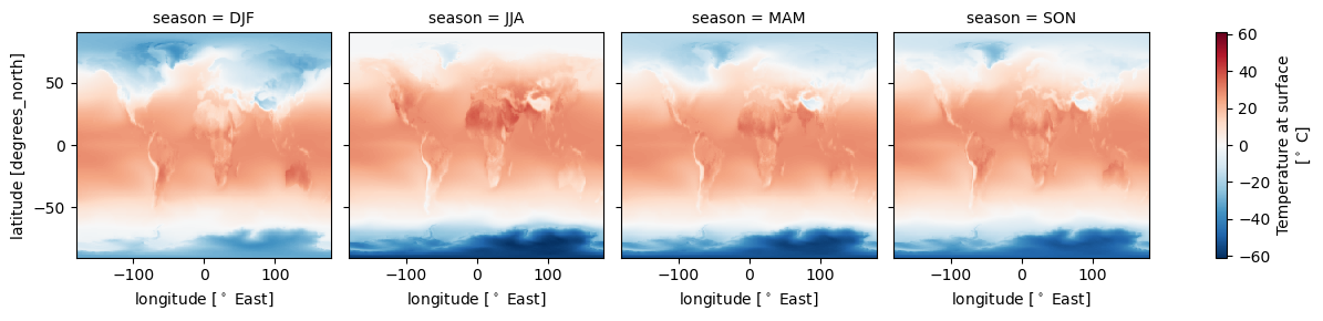
Tip: Might want to load or compute.

from dask.diagnostics import ProgressBar

%%time
with ProgressBar():
    da_TC.load()

[########################################] | 100% Completed | 3.32 ss
CPU times: user 910 ms, sys: 256 ms, total: 1.17 s
Wall time: 3.33 s

10. Controle the plot visuals:

%%time
da_TC.plot(
    col = 'season',
    cmap = 'coolwarm',
    xlim = [-100,100],
    ylim = [-0,90],
    cbar_kwargs = {'label':'Temperature [$^\circ$C]'}
    )

CPU times: user 151 ms, sys: 3.23 ms, total: 155 ms
Wall time: 154 ms

<unknown>:6: SyntaxWarning: invalid escape sequence '\c'

<xarray.plot.facetgrid.FacetGrid at 0x7f7dc79df050>

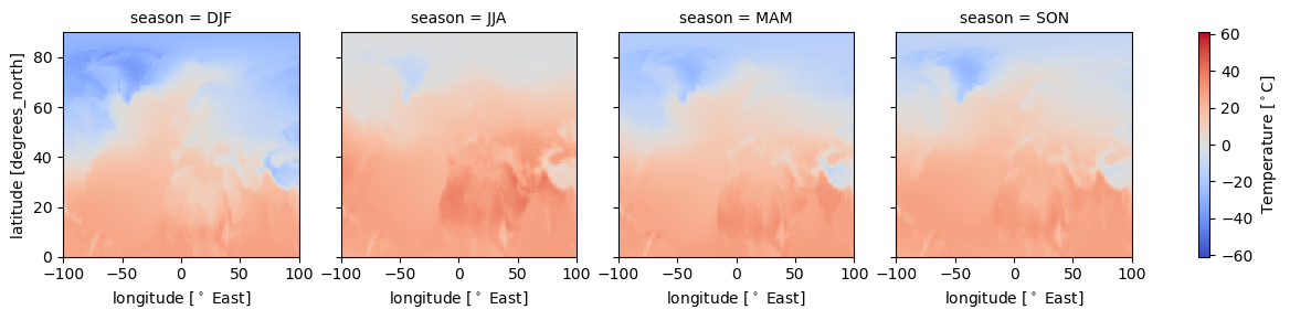
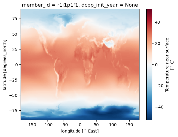
• Xarray uses certain attributes as labels when plotting:

da_TC = da_TC.assign_attrs({'long_name': 'Temperature near surface'})

da_TC.mean('season', keep_attrs=True).plot()

<matplotlib.collections.QuadMesh at 0x7f7dc7649cd0>

11. Plotting on maps with cartopy

See more here:

• Plotting with xarray

• Plotting with cartopy and xarray

• Cartopy projection list

import cartopy as cy
import cartopy.crs as ccrs

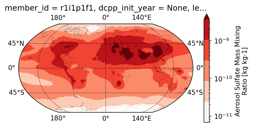
da_plt = dss['mmrso4'].isel(lev=-1).mean('time', keep_attrs=True).squeeze()#('member_id')

da_plt

<xarray.DataArray 'mmrso4' (lat: 192, lon: 288)> Size: 221kB
dask.array<getitem, shape=(192, 288), dtype=float32, chunksize=(192, 288), chunktype=numpy.ndarray>
Coordinates:
  * lat             (lat) float64 2kB -90.0 -89.06 -88.12 ... 88.12 89.06 90.0
  * lon             (lon) float64 2kB -180.0 -178.8 -177.5 ... 176.2 177.5 178.8
    member_id       <U8 32B 'r1i1p1f1'
    dcpp_init_year  object 8B None
    lev             float64 8B -992.6
Attributes: (12/19)
    cell_measures:  area: areacella
    cell_methods:   area: time: mean
    comment:        Dry mass of sulfate (SO4) in aerosol particles as a fract...
    description:    Dry mass of sulfate (SO4) in aerosol particles as a fract...
    frequency:      mon
    id:             mmrso4
    ...             ...
    time_label:     time-mean
    time_title:     Temporal mean
    title:          Aerosol Sulfate Mass Mixing Ratio
    type:           real
    units:          kg kg-1
    variable_id:    mmrso4

xarray.DataArray

'mmrso4'

• lat: 192
• lon: 288

• dask.array<chunksize=(192, 288), meta=np.ndarray>

  Array Chunk Bytes 216.00 kiB 216.00 kiB Shape (192, 288) (192, 288) Dask graph 1 chunks in 11 graph layers Data type float32 numpy.ndarray

• Coordinates: (5)
  • lat
    (lat)
    float64
    -90.0 -89.06 -88.12 ... 89.06 90.0

    axis :

    Y

    bounds :

    lat_bnds

    standard_name :

    latitude

    title :

    Latitude

    type :

    double

    units :

    degrees_north

    valid_max :

    90.0

    valid_min :

    -90.0

    array([-90.      , -89.057592, -88.115183, -87.172775, -86.230366, -85.287958,
           -84.34555 , -83.403141, -82.460733, -81.518325, -80.575916, -79.633508,
           -78.691099, -77.748691, -76.806283, -75.863874, -74.921466, -73.979058,
           -73.036649, -72.094241, -71.151832, -70.209424, -69.267016, -68.324607,
           -67.382199, -66.439791, -65.497382, -64.554974, -63.612565, -62.670157,
           -61.727749, -60.78534 , -59.842932, -58.900524, -57.958115, -57.015707,
           -56.073298, -55.13089 , -54.188482, -53.246073, -52.303665, -51.361257,
           -50.418848, -49.47644 , -48.534031, -47.591623, -46.649215, -45.706806,
           -44.764398, -43.82199 , -42.879581, -41.937173, -40.994764, -40.052356,
           -39.109948, -38.167539, -37.225131, -36.282723, -35.340314, -34.397906,
           -33.455497, -32.513089, -31.570681, -30.628272, -29.685864, -28.743455,
           -27.801047, -26.858639, -25.91623 , -24.973822, -24.031414, -23.089005,
           -22.146597, -21.204188, -20.26178 , -19.319372, -18.376963, -17.434555,
           -16.492147, -15.549738, -14.60733 , -13.664921, -12.722513, -11.780105,
           -10.837696,  -9.895288,  -8.95288 ,  -8.010471,  -7.068063,  -6.125654,
            -5.183246,  -4.240838,  -3.298429,  -2.356021,  -1.413613,  -0.471204,
             0.471204,   1.413613,   2.356021,   3.298429,   4.240838,   5.183246,
             6.125654,   7.068063,   8.010471,   8.95288 ,   9.895288,  10.837696,
            11.780105,  12.722513,  13.664921,  14.60733 ,  15.549738,  16.492147,
            17.434555,  18.376963,  19.319372,  20.26178 ,  21.204188,  22.146597,
            23.089005,  24.031414,  24.973822,  25.91623 ,  26.858639,  27.801047,
            28.743455,  29.685864,  30.628272,  31.570681,  32.513089,  33.455497,
            34.397906,  35.340314,  36.282723,  37.225131,  38.167539,  39.109948,
            40.052356,  40.994764,  41.937173,  42.879581,  43.82199 ,  44.764398,
            45.706806,  46.649215,  47.591623,  48.534031,  49.47644 ,  50.418848,
            51.361257,  52.303665,  53.246073,  54.188482,  55.13089 ,  56.073298,
            57.015707,  57.958115,  58.900524,  59.842932,  60.78534 ,  61.727749,
            62.670157,  63.612565,  64.554974,  65.497382,  66.439791,  67.382199,
            68.324607,  69.267016,  70.209424,  71.151832,  72.094241,  73.036649,
            73.979058,  74.921466,  75.863874,  76.806283,  77.748691,  78.691099,
            79.633508,  80.575916,  81.518325,  82.460733,  83.403141,  84.34555 ,
            85.287958,  86.230366,  87.172775,  88.115183,  89.057592,  90.      ])

  • lon
    (lon)
    float64
    -180.0 -178.8 ... 177.5 178.8

    axis :

    X

    bounds :

    lon_bnds

    standard_name :

    longitude

    title :

    Longitude

    type :

    double

    units :

    $^\circ$ East

    valid_max :

    360.0

    valid_min :

    0.0

    array([-180.  , -178.75, -177.5 , ...,  176.25,  177.5 ,  178.75], shape=(288,))

  • member_id
    ()
    <U8
    'r1i1p1f1'

    array('r1i1p1f1', dtype='<U8')

  • dcpp_init_year
    ()
    object
    None

    array(None, dtype=object)

  • lev
    ()
    float64
    -992.6

    axis :

    Z

    bounds :

    lev_bnds

    positive :

    up

    standard_name :

    alevel

    title :

    atmospheric model level

    type :

    double

    units :

    hPa

    array(-992.55609512)

• Attributes: (19)

  cell_measures :

  area: areacella

  cell_methods :

  area: time: mean

  comment :

  Dry mass of sulfate (SO4) in aerosol particles as a fraction of air mass.

  description :

  Dry mass of sulfate (SO4) in aerosol particles as a fraction of air mass.

  frequency :

  mon

  id :

  mmrso4

  long_name :

  Aerosol Sulfate Mass Mixing Ratio

  mipTable :

  AERmon

  out_name :

  mmrso4

  prov :

  AERmon ((isd.003))

  realm :

  aerosol

  standard_name :

  mass_fraction_of_sulfate_dry_aerosol_particles_in_air

  time :

  time

  time_label :

  time-mean

  time_title :

  Temporal mean

  title :

  Aerosol Sulfate Mass Mixing Ratio

  type :

  real

  units :

  kg kg-1

  variable_id :

  mmrso4

from matplotlib.colors import LogNorm

with ProgressBar():
    da_plt.load()

[########################################] | 100% Completed | 15.82 s

da_plt

<xarray.DataArray 'mmrso4' (lat: 192, lon: 288)> Size: 221kB
array([[7.0655860e-12, 7.0656250e-12, 7.0656757e-12, ..., 7.0654576e-12,
        7.0654355e-12, 7.0655361e-12],
       [7.4523243e-12, 7.4701807e-12, 7.4873970e-12, ..., 7.3945355e-12,
        7.4097612e-12, 7.4321209e-12],
       [8.0703352e-12, 8.0987569e-12, 8.1331625e-12, ..., 7.9838211e-12,
        8.0185901e-12, 8.0491074e-12],
       ...,
       [3.2195208e-11, 3.2224824e-11, 3.2185154e-11, ..., 3.2204971e-11,
        3.2198522e-11, 3.2200648e-11],
       [3.1399085e-11, 3.1360515e-11, 3.1390588e-11, ..., 3.1466201e-11,
        3.1436742e-11, 3.1405469e-11],
       [3.0563073e-11, 3.0563111e-11, 3.0562844e-11, ..., 3.0563923e-11,
        3.0565089e-11, 3.0564860e-11]], shape=(192, 288), dtype=float32)
Coordinates:
  * lat             (lat) float64 2kB -90.0 -89.06 -88.12 ... 88.12 89.06 90.0
  * lon             (lon) float64 2kB -180.0 -178.8 -177.5 ... 176.2 177.5 178.8
    member_id       <U8 32B 'r1i1p1f1'
    dcpp_init_year  object 8B None
    lev             float64 8B -992.6
Attributes: (12/19)
    cell_measures:  area: areacella
    cell_methods:   area: time: mean
    comment:        Dry mass of sulfate (SO4) in aerosol particles as a fract...
    description:    Dry mass of sulfate (SO4) in aerosol particles as a fract...
    frequency:      mon
    id:             mmrso4
    ...             ...
    time_label:     time-mean
    time_title:     Temporal mean
    title:          Aerosol Sulfate Mass Mixing Ratio
    type:           real
    units:          kg kg-1
    variable_id:    mmrso4

xarray.DataArray

'mmrso4'

• lat: 192
• lon: 288

• 7.066e-12 7.066e-12 7.066e-12 ... 3.056e-11 3.057e-11 3.056e-11

  array([[7.0655860e-12, 7.0656250e-12, 7.0656757e-12, ..., 7.0654576e-12,
          7.0654355e-12, 7.0655361e-12],
         [7.4523243e-12, 7.4701807e-12, 7.4873970e-12, ..., 7.3945355e-12,
          7.4097612e-12, 7.4321209e-12],
         [8.0703352e-12, 8.0987569e-12, 8.1331625e-12, ..., 7.9838211e-12,
          8.0185901e-12, 8.0491074e-12],
         ...,
         [3.2195208e-11, 3.2224824e-11, 3.2185154e-11, ..., 3.2204971e-11,
          3.2198522e-11, 3.2200648e-11],
         [3.1399085e-11, 3.1360515e-11, 3.1390588e-11, ..., 3.1466201e-11,
          3.1436742e-11, 3.1405469e-11],
         [3.0563073e-11, 3.0563111e-11, 3.0562844e-11, ..., 3.0563923e-11,
          3.0565089e-11, 3.0564860e-11]], shape=(192, 288), dtype=float32)

• Coordinates: (5)
  • lat
    (lat)
    float64
    -90.0 -89.06 -88.12 ... 89.06 90.0

    axis :

    Y

    bounds :

    lat_bnds

    standard_name :

    latitude

    title :

    Latitude

    type :

    double

    units :

    degrees_north

    valid_max :

    90.0

    valid_min :

    -90.0

    array([-90.      , -89.057592, -88.115183, -87.172775, -86.230366, -85.287958,
           -84.34555 , -83.403141, -82.460733, -81.518325, -80.575916, -79.633508,
           -78.691099, -77.748691, -76.806283, -75.863874, -74.921466, -73.979058,
           -73.036649, -72.094241, -71.151832, -70.209424, -69.267016, -68.324607,
           -67.382199, -66.439791, -65.497382, -64.554974, -63.612565, -62.670157,
           -61.727749, -60.78534 , -59.842932, -58.900524, -57.958115, -57.015707,
           -56.073298, -55.13089 , -54.188482, -53.246073, -52.303665, -51.361257,
           -50.418848, -49.47644 , -48.534031, -47.591623, -46.649215, -45.706806,
           -44.764398, -43.82199 , -42.879581, -41.937173, -40.994764, -40.052356,
           -39.109948, -38.167539, -37.225131, -36.282723, -35.340314, -34.397906,
           -33.455497, -32.513089, -31.570681, -30.628272, -29.685864, -28.743455,
           -27.801047, -26.858639, -25.91623 , -24.973822, -24.031414, -23.089005,
           -22.146597, -21.204188, -20.26178 , -19.319372, -18.376963, -17.434555,
           -16.492147, -15.549738, -14.60733 , -13.664921, -12.722513, -11.780105,
           -10.837696,  -9.895288,  -8.95288 ,  -8.010471,  -7.068063,  -6.125654,
            -5.183246,  -4.240838,  -3.298429,  -2.356021,  -1.413613,  -0.471204,
             0.471204,   1.413613,   2.356021,   3.298429,   4.240838,   5.183246,
             6.125654,   7.068063,   8.010471,   8.95288 ,   9.895288,  10.837696,
            11.780105,  12.722513,  13.664921,  14.60733 ,  15.549738,  16.492147,
            17.434555,  18.376963,  19.319372,  20.26178 ,  21.204188,  22.146597,
            23.089005,  24.031414,  24.973822,  25.91623 ,  26.858639,  27.801047,
            28.743455,  29.685864,  30.628272,  31.570681,  32.513089,  33.455497,
            34.397906,  35.340314,  36.282723,  37.225131,  38.167539,  39.109948,
            40.052356,  40.994764,  41.937173,  42.879581,  43.82199 ,  44.764398,
            45.706806,  46.649215,  47.591623,  48.534031,  49.47644 ,  50.418848,
            51.361257,  52.303665,  53.246073,  54.188482,  55.13089 ,  56.073298,
            57.015707,  57.958115,  58.900524,  59.842932,  60.78534 ,  61.727749,
            62.670157,  63.612565,  64.554974,  65.497382,  66.439791,  67.382199,
            68.324607,  69.267016,  70.209424,  71.151832,  72.094241,  73.036649,
            73.979058,  74.921466,  75.863874,  76.806283,  77.748691,  78.691099,
            79.633508,  80.575916,  81.518325,  82.460733,  83.403141,  84.34555 ,
            85.287958,  86.230366,  87.172775,  88.115183,  89.057592,  90.      ])

  • lon
    (lon)
    float64
    -180.0 -178.8 ... 177.5 178.8

    axis :

    X

    bounds :

    lon_bnds

    standard_name :

    longitude

    title :

    Longitude

    type :

    double

    units :

    $^\circ$ East

    valid_max :

    360.0

    valid_min :

    0.0

    array([-180.  , -178.75, -177.5 , ...,  176.25,  177.5 ,  178.75], shape=(288,))

  • member_id
    ()
    <U8
    'r1i1p1f1'

    array('r1i1p1f1', dtype='<U8')

  • dcpp_init_year
    ()
    object
    None

    array(None, dtype=object)

  • lev
    ()
    float64
    -992.6

    axis :

    Z

    bounds :

    lev_bnds

    positive :

    up

    standard_name :

    alevel

    title :

    atmospheric model level

    type :

    double

    units :

    hPa

    array(-992.55609512)

• Attributes: (19)

  cell_measures :

  area: areacella

  cell_methods :

  area: time: mean

  comment :

  Dry mass of sulfate (SO4) in aerosol particles as a fraction of air mass.

  description :

  Dry mass of sulfate (SO4) in aerosol particles as a fraction of air mass.

  frequency :

  mon

  id :

  mmrso4

  long_name :

  Aerosol Sulfate Mass Mixing Ratio

  mipTable :

  AERmon

  out_name :

  mmrso4

  prov :

  AERmon ((isd.003))

  realm :

  aerosol

  standard_name :

  mass_fraction_of_sulfate_dry_aerosol_particles_in_air

  time :

  time

  time_label :

  time-mean

  time_title :

  Temporal mean

  title :

  Aerosol Sulfate Mass Mixing Ratio

  type :

  real

  units :

  kg kg-1

  variable_id :

  mmrso4

• projection tells cartopy how we want the data visualized

• transform tells it what kind of grid the data is on:

  • PlateCarree is a regular lat, lon grid.

Note to Sara: robust, LogNorm, cbar_kwargs, levels

f, ax = plt.subplots(1, 1, dpi=150, figsize = [6,3],
                    subplot_kw={'projection':ccrs.Robinson()},
                    #subplot_kw={'projection':ccrs.Orthographic()},
                   )

da_plt.plot.pcolormesh(
    cmap = 'Reds',
    ax=ax,
    transform = ccrs.PlateCarree(), 
    robust=True,
    norm = LogNorm(), # to add log scale colorbar
    #cbar_kwargs={
    #    #'label':'Wind Speed [m/s]', 
    #    'orientation':'horizontal',
    #    'shrink':.8
    #},
    levels = 6
)
#ax.set_title('Bottom level: Mean over Time')


ax.coastlines(linewidth=.1)
gl = ax.gridlines(draw_labels=True,#{'bottom':True, 'left':True},
                  xlocs=[-180,-140,0,140, 180],
                  ylocs=[-90,-45,0,45,90],
                  x_inline=False,
                  y_inline=False,
                  color='k',
                  linestyle='dotted'
                 )

12. Global average: weighted means!

dss['T_C'].mean().compute()

<xarray.DataArray 'T_C' ()> Size: 4B
array(5.4478564, dtype=float32)
Attributes: (12/19)
    cell_measures:  area: areacella
    cell_methods:   area: time: mean
    comment:        near-surface (usually, 2 meter) air temperature
    description:    near-surface (usually, 2 meter) air temperature
    frequency:      mon
    id:             tas
    ...             ...
    time_label:     time-mean
    time_title:     Temporal mean
    title:          Near-Surface Air Temperature
    type:           real
    units:          $^\circ$ C
    variable_id:    tas

xarray.DataArray

'T_C'

• 5.448

  array(5.4478564, dtype=float32)

• Attributes: (19)

  cell_measures :

  area: areacella

  cell_methods :

  area: time: mean

  comment :

  near-surface (usually, 2 meter) air temperature

  description :

  near-surface (usually, 2 meter) air temperature

  frequency :

  mon

  id :

  tas

  long_name :

  Temperature at surface

  mipTable :

  Amon

  out_name :

  tas

  prov :

  Amon ((isd.003))

  realm :

  atmos

  standard_name :

  air_temperature

  time :

  time

  time_label :

  time-mean

  time_title :

  Temporal mean

  title :

  Near-Surface Air Temperature

  type :

  real

  units :

  $^\circ$ C

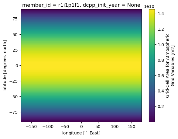
  variable_id :

  tas

Why is this wrong?

(dss['T_C']
    .weighted(dss['areacella'])
    .mean()
    .compute()
)

<xarray.DataArray 'T_C' ()> Size: 4B
array(14.715101, dtype=float32)
Attributes: (12/19)
    cell_measures:  area: areacella
    cell_methods:   area: time: mean
    comment:        near-surface (usually, 2 meter) air temperature
    description:    near-surface (usually, 2 meter) air temperature
    frequency:      mon
    id:             tas
    ...             ...
    time_label:     time-mean
    time_title:     Temporal mean
    title:          Near-Surface Air Temperature
    type:           real
    units:          $^\circ$ C
    variable_id:    tas

xarray.DataArray

'T_C'

• 14.72

  array(14.715101, dtype=float32)

• Attributes: (19)

  cell_measures :

  area: areacella

  cell_methods :

  area: time: mean

  comment :

  near-surface (usually, 2 meter) air temperature

  description :

  near-surface (usually, 2 meter) air temperature

  frequency :

  mon

  id :

  tas

  long_name :

  Temperature at surface

  mipTable :

  Amon

  out_name :

  tas

  prov :

  Amon ((isd.003))

  realm :

  atmos

  standard_name :

  air_temperature

  time :

  time

  time_label :

  time-mean

  time_title :

  Temporal mean

  title :

  Near-Surface Air Temperature

  type :

  real

  units :

  $^\circ$ C

  variable_id :

  tas

dss['areacella'].plot()

<matplotlib.collections.QuadMesh at 0x7f7ea8e70f50>

13 Filtering, grouping etc

Pick out station:

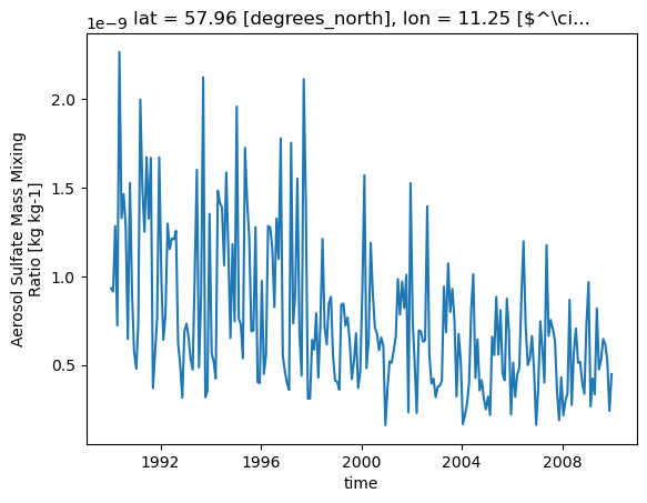
lat_kristineberg = 58.24
lon_kristineberg = 11.44
# pick out surface
ds_surf =dss.isel(lev=-1)
ds_kristineberg = ds_surf.sel(lat=lat_kristineberg, lon = lon_kristineberg, method ='nearest')

ds_kristineberg['mmrso4'].plot()

[<matplotlib.lines.Line2D at 0x7f7ea8fac230>]

Pick out the vairables we need.

with ProgressBar():
    ds_kristineberg.load()

[########################################] | 100% Completed | 18.64 ss

vl = ['mmrso4','hurs','tas','T_C']

ds_kristineberg[vl]

<xarray.Dataset> Size: 6kB
Dimensions:         (member_id: 1, dcpp_init_year: 1, time: 240)
Coordinates:
  * member_id       (member_id) object 8B 'r1i1p1f1'
  * dcpp_init_year  (dcpp_init_year) object 8B None
  * time            (time) datetime64[ns] 2kB 1990-01-15T12:00:00 ... 2009-12...
    lat             float64 8B 57.96
    lon             float64 8B 11.25
    lev             float64 8B -992.6
Data variables:
    mmrso4          (member_id, dcpp_init_year, time) float32 960B 9.319e-10 ...
    hurs            (member_id, dcpp_init_year, time) float32 960B 85.65 ... ...
    tas             (member_id, dcpp_init_year, time) float32 960B 277.0 ... ...
    T_C             (member_id, dcpp_init_year, time) float32 960B 3.886 ... ...
Attributes: (12/58)
    Conventions:                      CF-1.7 CMIP-6.2
    activity_id:                      CMIP
    branch_method:                    standard
    branch_time_in_child:             674885.0
    branch_time_in_parent:            219000.0
    case_id:                          15
    ...                               ...
    intake_esm_attrs:variable_id:     areacella
    intake_esm_attrs:grid_label:      gn
    intake_esm_attrs:zstore:          gs://cmip6/CMIP6/CMIP/NCAR/CESM2/histor...
    intake_esm_attrs:version:         20190308
    intake_esm_attrs:_data_format_:   zarr
    intake_esm_dataset_key:           CMIP.historical.CESM2.fx.gn

xarray.Dataset

• Dimensions:
  • member_id: 1
  • dcpp_init_year: 1
  • time: 240
• Coordinates: (6)
  • member_id
    (member_id)
    object
    'r1i1p1f1'

    array(['r1i1p1f1'], dtype=object)

  • dcpp_init_year
    (dcpp_init_year)
    object
    None

    array([None], dtype=object)

  • time
    (time)
    datetime64[ns]
    1990-01-15T12:00:00 ... 2009-12-...

    array(['1990-01-15T12:00:00.000000000', '1990-02-14T00:00:00.000000000',
           '1990-03-15T12:00:00.000000000', ..., '2009-10-15T12:00:00.000000000',
           '2009-11-15T00:00:00.000000000', '2009-12-15T12:00:00.000000000'],
          shape=(240,), dtype='datetime64[ns]')

  • lat
    ()
    float64
    57.96

    axis :

    Y

    bounds :

    lat_bnds

    standard_name :

    latitude

    title :

    Latitude

    type :

    double

    units :

    degrees_north

    valid_max :

    90.0

    valid_min :

    -90.0

    array(57.95811518)

  • lon
    ()
    float64
    11.25

    axis :

    X

    bounds :

    lon_bnds

    standard_name :

    longitude

    title :

    Longitude

    type :

    double

    units :

    $^\circ$ East

    valid_max :

    360.0

    valid_min :

    0.0

    array(11.25)

  • lev
    ()
    float64
    -992.6

    axis :

    Z

    bounds :

    lev_bnds

    positive :

    up

    standard_name :

    alevel

    title :

    atmospheric model level

    type :

    double

    units :

    hPa

    array(-992.55609512)

• Data variables: (4)
  • mmrso4
    (member_id, dcpp_init_year, time)
    float32
    9.319e-10 9.139e-10 ... 4.485e-10

    cell_measures :

    area: areacella

    cell_methods :

    area: time: mean

    comment :

    Dry mass of sulfate (SO4) in aerosol particles as a fraction of air mass.

    description :

    Dry mass of sulfate (SO4) in aerosol particles as a fraction of air mass.

    frequency :

    mon

    id :

    mmrso4

    long_name :

    Aerosol Sulfate Mass Mixing Ratio

    mipTable :

    AERmon

    out_name :

    mmrso4

    prov :

    AERmon ((isd.003))

    realm :

    aerosol

    standard_name :

    mass_fraction_of_sulfate_dry_aerosol_particles_in_air

    time :

    time

    time_label :

    time-mean

    time_title :

    Temporal mean

    title :

    Aerosol Sulfate Mass Mixing Ratio

    type :

    real

    units :

    kg kg-1

    variable_id :

    mmrso4

    array([[[9.3193886e-10, 9.1392072e-10, 1.2826715e-09, 7.2257367e-10,
             2.2636457e-09, 1.3281619e-09, 1.4629278e-09, 1.2863141e-09,
             6.4677341e-10, 1.5266306e-09, 9.0736763e-10, 5.7557659e-10,
             4.7942467e-10, 7.3377227e-10, 1.9957693e-09, 1.4964732e-09,
             1.2506074e-09, 1.6712218e-09, 1.3250209e-09, 1.6674845e-09,
             3.6972247e-10, 5.6149579e-10, 7.6491025e-10, 1.6698171e-09,
             9.8607511e-10, 6.4137351e-10, 7.8463064e-10, 1.2971688e-09,
             1.1532616e-09, 1.2129736e-09, 1.2082786e-09, 1.2557465e-09,
             6.2253258e-10, 5.0003912e-10, 3.1542999e-10, 6.8933742e-10,
             7.3369416e-10, 6.5658307e-10, 5.3543248e-10, 4.7376575e-10,
             1.0168403e-09, 1.6001662e-09, 4.8634125e-10, 8.9594443e-10,
             2.1212649e-09, 3.1811920e-10, 3.5666189e-10, 1.3520196e-09,
             5.6667299e-10, 5.1949695e-10, 4.2386877e-10, 1.4821199e-09,
             1.4134094e-09, 1.3894664e-09, 1.0615168e-09, 1.5850201e-09,
             1.1513889e-09, 6.5186895e-10, 1.1817154e-09, 7.4557799e-10,
             1.9564568e-09, 7.6402235e-10, 7.2592093e-10, 5.3814297e-10,
             1.7240011e-09, 1.4250184e-09, 1.2221594e-09, 6.8972605e-10,
             6.9383221e-10, 1.2773098e-09, 4.0283718e-10, 3.9811388e-10,
             9.7333863e-10, 4.4941270e-10, 5.5883020e-10, 1.2838162e-09,
             1.2748105e-09, 1.1566451e-09, 8.2630669e-10, 1.3249776e-09,
    ...
             7.5434198e-10, 3.2416719e-10, 6.7540507e-10, 5.2173044e-10,
             1.6671606e-10, 2.1651315e-10, 2.7970151e-10, 3.9993286e-10,
             8.1241042e-10, 1.0122931e-09, 4.2739132e-10, 6.4456152e-10,
             3.5591874e-10, 4.1421538e-10, 3.1068517e-10, 2.5002367e-10,
             3.2186834e-10, 2.1786670e-10, 6.5897471e-10, 5.5566390e-10,
             8.8390589e-10, 5.5829497e-10, 8.0862272e-10, 4.4708118e-10,
             4.1382620e-10, 8.7374258e-10, 6.8856332e-10, 2.2117561e-10,
             5.1323434e-10, 3.2079947e-10, 4.4620288e-10, 4.8293736e-10,
             8.8299312e-10, 1.1971121e-09, 7.2521211e-10, 4.9940829e-10,
             5.3397714e-10, 6.6344513e-10, 4.7186260e-10, 1.6243321e-10,
             3.7509162e-10, 7.4617806e-10, 5.9407895e-10, 4.0051451e-10,
             1.1766452e-09, 6.6410638e-10, 7.5369005e-10, 7.0132800e-10,
             6.3694217e-10, 3.4894496e-10, 1.8863487e-10, 4.3067430e-10,
             2.1598053e-10, 2.9836339e-10, 3.3995992e-10, 8.6714907e-10,
             2.7420552e-10, 5.7396254e-10, 7.0535694e-10, 5.1266724e-10,
             5.1790988e-10, 4.0158260e-10, 3.3728587e-10, 7.2649092e-10,
             9.6747377e-10, 2.6640706e-10, 4.2341586e-10, 3.3404060e-10,
             8.1849499e-10, 4.7471893e-10, 5.2741644e-10, 6.4691424e-10,
             6.1747668e-10, 5.2262034e-10, 2.4114855e-10, 4.4853779e-10]]],
          dtype=float32)

  • hurs
    (member_id, dcpp_init_year, time)
    float32
    85.65 79.78 82.47 ... 83.64 89.49

    cell_measures :

    area: areacella

    cell_methods :

    area: time: mean

    comment :

    This is the relative humidity with respect to liquid water for T> 0 C, and with respect to ice for T<0 C.

    description :

    This is the relative humidity with respect to liquid water for T> 0 C, and with respect to ice for T<0 C.

    frequency :

    mon

    id :

    hurs

    long_name :

    Near-Surface Relative Humidity

    mipTable :

    Amon

    out_name :

    hurs

    prov :

    Amon ((isd.003))

    realm :

    atmos

    standard_name :

    relative_humidity

    time :

    time

    time_label :

    time-mean

    time_title :

    Temporal mean

    title :

    Near-Surface Relative Humidity

    type :

    real

    units :

    %

    variable_id :

    hurs

    array([[[85.6512  , 79.7797  , 82.473785, 79.58873 , 80.421875,
             84.58708 , 84.94299 , 72.892365, 75.627266, 83.52159 ,
             81.26038 , 84.68246 , 81.28056 , 86.9214  , 84.940254,
             71.434   , 81.14642 , 84.55596 , 79.76721 , 82.525185,
             69.615944, 77.52233 , 79.28391 , 89.902054, 89.68583 ,
             86.76022 , 78.673225, 80.402504, 77.28582 , 86.062775,
             84.12753 , 81.188934, 72.5107  , 78.06689 , 79.50622 ,
             85.14791 , 85.16971 , 79.308556, 81.106255, 74.15938 ,
             76.85091 , 83.09885 , 80.1934  , 77.61525 , 81.34912 ,
             74.56923 , 81.82556 , 86.91707 , 84.77872 , 79.13002 ,
             70.701294, 76.79796 , 81.3291  , 81.01642 , 84.95078 ,
             80.43662 , 78.639725, 79.71097 , 82.36563 , 82.5781  ,
             86.097916, 77.24076 , 84.35341 , 76.216255, 82.4589  ,
             83.908615, 81.38897 , 79.03039 , 76.288734, 81.49444 ,
             83.08849 , 81.42568 , 88.53188 , 85.09241 , 77.77556 ,
             79.70282 , 80.305466, 83.2992  , 80.25415 , 81.289894,
             80.31601 , 86.42468 , 79.22198 , 80.783966, 85.659645,
             82.79457 , 83.75577 , 83.89612 , 87.54124 , 85.52979 ,
             84.52526 , 78.82385 , 83.94702 , 80.09471 , 82.58052 ,
             85.81947 , 88.3496  , 81.24771 , 81.73555 , 80.737564,
    ...
             86.58703 , 77.65002 , 76.92285 , 82.098526, 81.421104,
             81.656944, 85.26446 , 76.72732 , 78.53415 , 84.1566  ,
             83.29057 , 81.94568 , 78.68756 , 75.4941  , 73.73777 ,
             83.86288 , 83.008995, 80.959   , 78.48728 , 77.348274,
             76.765884, 82.4043  , 84.123245, 84.66348 , 77.667564,
             80.34306 , 74.82629 , 81.81224 , 84.970146, 80.859344,
             80.14923 , 73.6474  , 82.12172 , 83.96776 , 83.2338  ,
             83.37189 , 81.97976 , 77.62364 , 84.172966, 84.03998 ,
             79.95671 , 84.44249 , 76.10524 , 79.596825, 81.99454 ,
             85.85605 , 80.008606, 80.301796, 83.00442 , 82.715614,
             77.42871 , 81.817406, 86.23183 , 81.13182 , 81.60189 ,
             75.99792 , 80.1371  , 81.668274, 80.24692 , 85.04006 ,
             85.7113  , 83.677536, 69.43945 , 83.40899 , 83.40006 ,
             85.41751 , 84.303856, 77.21337 , 77.8262  , 76.52623 ,
             82.73933 , 86.96575 , 83.560455, 79.949036, 78.34009 ,
             71.88216 , 82.32212 , 82.4355  , 77.32013 , 80.14359 ,
             80.89918 , 79.335236, 84.31219 , 89.36123 , 84.628136,
             79.660576, 71.35938 , 79.27945 , 82.85541 , 79.48341 ,
             82.33854 , 75.105225, 81.02953 , 83.64138 , 89.48721 ]]],
          dtype=float32)

  • tas
    (member_id, dcpp_init_year, time)
    float32
    277.0 273.6 277.4 ... 278.7 277.5

    cell_measures :

    area: areacella

    cell_methods :

    area: time: mean

    comment :

    near-surface (usually, 2 meter) air temperature

    description :

    near-surface (usually, 2 meter) air temperature

    frequency :

    mon

    id :

    tas

    long_name :

    Near-Surface Air Temperature

    mipTable :

    Amon

    out_name :

    tas

    prov :

    Amon ((isd.003))

    realm :

    atmos

    standard_name :

    air_temperature

    time :

    time

    time_label :

    time-mean

    time_title :

    Temporal mean

    title :

    Near-Surface Air Temperature

    type :

    real

    units :

    K

    variable_id :

    tas

    array([[[277.036  , 273.6018 , 277.4057 , 280.13733, 283.04315,
             286.1976 , 288.96158, 288.67313, 286.447  , 282.331  ,
             280.6072 , 277.33212, 276.35056, 275.45718, 278.24026,
             278.6902 , 282.02042, 287.577  , 289.411  , 289.88937,
             286.20694, 283.30524, 278.37958, 274.88986, 275.9685 ,
             273.18692, 273.93338, 277.60355, 280.31152, 285.03375,
             287.31808, 288.47113, 285.9238 , 282.57498, 275.49026,
             275.0295 , 277.4612 , 276.80396, 278.17105, 278.80664,
             281.17633, 286.22424, 286.43982, 286.2223 , 286.87054,
             280.75034, 281.23383, 278.1589 , 279.02744, 276.0177 ,
             274.74112, 278.6569 , 282.93082, 286.23575, 290.3751 ,
             289.93   , 287.68118, 285.75076, 282.43347, 280.83716,
             276.75778, 274.70197, 277.61902, 279.36847, 282.76617,
             286.89862, 287.75464, 288.02655, 286.36737, 283.76627,
             281.2449 , 278.22116, 275.7414 , 272.185  , 274.5559 ,
             278.77332, 282.7405 , 287.1005 , 287.9257 , 289.6798 ,
             287.99744, 285.52274, 282.72733, 277.2558 , 275.17532,
             277.2748 , 278.09113, 280.724  , 283.00928, 286.29123,
             288.06375, 288.2159 , 288.11716, 282.65875, 280.7434 ,
             279.24933, 279.11615, 277.5452 , 277.96658, 280.3044 ,
    ...
             276.63882, 278.0943 , 278.8853 , 282.86172, 286.525  ,
             288.575  , 290.84235, 287.7864 , 286.16046, 282.43958,
             278.81308, 277.3345 , 277.58786, 276.546  , 278.729  ,
             283.8123 , 287.2157 , 289.00388, 290.0209 , 288.48395,
             284.43906, 280.91425, 277.32306, 277.92804, 276.23212,
             277.96164, 279.61298, 283.68323, 287.7096 , 288.3466 ,
             289.01794, 286.41257, 283.7271 , 279.47147, 280.5569 ,
             279.27786, 279.0786 , 278.42728, 280.98596, 284.1375 ,
             286.53778, 289.71893, 289.15417, 287.5555 , 284.9453 ,
             282.5847 , 278.54913, 276.3146 , 276.473  , 278.11572,
             281.2289 , 283.62564, 287.56595, 288.81967, 289.9035 ,
             287.19138, 284.7344 , 280.03235, 278.63467, 275.95413,
             276.34845, 276.56122, 276.8956 , 282.77957, 287.18732,
             288.75058, 290.00266, 288.32962, 283.43085, 280.71335,
             275.38644, 277.57248, 275.94055, 277.2333 , 278.06137,
             281.24808, 284.98416, 288.2797 , 289.20377, 286.846  ,
             284.86862, 279.29944, 278.14166, 278.26358, 277.8097 ,
             278.3669 , 277.93552, 283.2631 , 286.61642, 288.55844,
             290.29236, 288.50214, 284.51822, 278.70798, 277.5374 ]]],
          dtype=float32)

  • T_C
    (member_id, dcpp_init_year, time)
    float32
    3.886 0.4518 4.256 ... 5.558 4.387

    cell_measures :

    area: areacella

    cell_methods :

    area: time: mean

    comment :

    near-surface (usually, 2 meter) air temperature

    description :

    near-surface (usually, 2 meter) air temperature

    frequency :

    mon

    id :

    tas

    long_name :

    Temperature at surface

    mipTable :

    Amon

    out_name :

    tas

    prov :

    Amon ((isd.003))

    realm :

    atmos

    standard_name :

    air_temperature

    time :

    time

    time_label :

    time-mean

    time_title :

    Temporal mean

    title :

    Near-Surface Air Temperature

    type :

    real

    units :

    $^\circ$ C

    variable_id :

    tas

    array([[[ 3.8860168 ,  0.45181274,  4.255707  ,  6.987335  ,
              9.893158  , 13.047607  , 15.811584  , 15.523132  ,
             13.296997  ,  9.181     ,  7.4572144 ,  4.182129  ,
              3.2005615 ,  2.30719   ,  5.090271  ,  5.5401917 ,
              8.870422  , 14.427002  , 16.261017  , 16.73938   ,
             13.056946  , 10.155243  ,  5.2295837 ,  1.7398682 ,
              2.818512  ,  0.03692627,  0.78338623,  4.4535522 ,
              7.1615295 , 11.883759  , 14.168091  , 15.321136  ,
             12.773804  ,  9.424988  ,  2.340271  ,  1.8795166 ,
              4.3112183 ,  3.6539612 ,  5.021057  ,  5.6566467 ,
              8.026337  , 13.074249  , 13.289825  , 13.072296  ,
             13.720551  ,  7.600342  ,  8.083832  ,  5.008911  ,
              5.8774414 ,  2.8677063 ,  1.5911255 ,  5.506897  ,
              9.780823  , 13.085754  , 17.225098  , 16.779999  ,
             14.531189  , 12.600769  ,  9.283478  ,  7.6871643 ,
              3.607788  ,  1.5519714 ,  4.4690247 ,  6.2184753 ,
              9.61618   , 13.748627  , 14.604645  , 14.876556  ,
             13.217377  , 10.616272  ,  8.09491   ,  5.071167  ,
              2.5914001 , -0.96499634,  1.4059143 ,  5.6233215 ,
              9.590515  , 13.9505005 , 14.775696  , 16.529816  ,
    ...
             15.333954  , 11.2890625 ,  7.7642517 ,  4.173065  ,
              4.7780457 ,  3.0821228 ,  4.8116455 ,  6.462982  ,
             10.533234  , 14.559601  , 15.196594  , 15.86795   ,
             13.262573  , 10.577118  ,  6.321472  ,  7.406891  ,
              6.1278687 ,  5.9286194 ,  5.2772827 ,  7.835968  ,
             10.987518  , 13.387787  , 16.56894   , 16.00418   ,
             14.405518  , 11.795319  ,  9.434692  ,  5.3991394 ,
              3.1646118 ,  3.322998  ,  4.9657288 ,  8.078918  ,
             10.475647  , 14.415955  , 15.669678  , 16.75351   ,
             14.041382  , 11.584412  ,  6.8823547 ,  5.48468   ,
              2.8041382 ,  3.1984558 ,  3.4112244 ,  3.7456055 ,
              9.629578  , 14.037323  , 15.600586  , 16.852661  ,
             15.179626  , 10.280853  ,  7.5633545 ,  2.2364502 ,
              4.4224854 ,  2.7905579 ,  4.083313  ,  4.911377  ,
              8.0980835 , 11.8341675 , 15.1297    , 16.053772  ,
             13.696014  , 11.718628  ,  6.1494446 ,  4.9916687 ,
              5.1135864 ,  4.6596985 ,  5.216919  ,  4.7855225 ,
             10.113098  , 13.466431  , 15.408447  , 17.142365  ,
             15.352142  , 11.368225  ,  5.5579834 ,  4.3874207 ]]],
          dtype=float32)

• Attributes: (58)

  Conventions :

  CF-1.7 CMIP-6.2

  activity_id :

  CMIP

  branch_method :

  standard

  branch_time_in_child :

  674885.0

  branch_time_in_parent :

  219000.0

  case_id :

  15

  cesm_casename :

  b.e21.BHIST.f09_g17.CMIP6-historical.001

  contact :

  cesm_cmip6@ucar.edu

  creation_date :

  2019-01-16T21:43:39Z

  data_specs_version :

  01.00.29

  experiment :

  all-forcing simulation of the recent past

  experiment_id :

  historical

  forcing_index :

  1

  frequency :

  fx

  further_info_url :

  https://furtherinfo.es-doc.org/CMIP6.NCAR.CESM2.historical.none.r1i1p1f1

  grid :

  native 0.9x1.25 finite volume grid (192x288 latxlon)

  grid_label :

  gn

  initialization_index :

  1

  institution :

  National Center for Atmospheric Research, Climate and Global Dynamics Laboratory, 1850 Table Mesa Drive, Boulder, CO 80305, USA

  institution_id :

  NCAR

  license :

  CMIP6 model data produced by <The National Center for Atmospheric Research> is licensed under a Creative Commons Attribution-[]ShareAlike 4.0 International License (https://creativecommons.org/licenses/). Consult https://pcmdi.llnl.gov/CMIP6/TermsOfUse for terms of use governing CMIP6 output, including citation requirements and proper acknowledgment. Further information about this data, including some limitations, can be found via the further_info_url (recorded as a global attribute in this file)[]. The data producers and data providers make no warranty, either express or implied, including, but not limited to, warranties of merchantability and fitness for a particular purpose. All liabilities arising from the supply of the information (including any liability arising in negligence) are excluded to the fullest extent permitted by law.

  mip_era :

  CMIP6

  model_doi_url :

  https://doi.org/10.5065/D67H1H0V

  nominal_resolution :

  100 km

  parent_activity_id :

  CMIP

  parent_experiment_id :

  piControl

  parent_mip_era :

  CMIP6

  parent_source_id :

  CESM2

  parent_time_units :

  days since 0001-01-01 00:00:00

  parent_variant_label :

  r1i1p1f1

  physics_index :

  1

  product :

  model-output

  realization_index :

  1

  realm :

  atmos land

  source :

  CESM2 (2017): atmosphere: CAM6 (0.9x1.25 finite volume grid; 288 x 192 longitude/latitude; 32 levels; top level 2.25 mb); ocean: POP2 (320x384 longitude/latitude; 60 levels; top grid cell 0-10 m); sea_ice: CICE5.1 (same grid as ocean); land: CLM5 0.9x1.25 finite volume grid; 288 x 192 longitude/latitude; 32 levels; top level 2.25 mb); aerosol: MAM4 (0.9x1.25 finite volume grid; 288 x 192 longitude/latitude; 32 levels; top level 2.25 mb); atmoschem: MAM4 (0.9x1.25 finite volume grid; 288 x 192 longitude/latitude; 32 levels; top level 2.25 mb); landIce: CISM2.1; ocnBgchem: MARBL (320x384 longitude/latitude; 60 levels; top grid cell 0-10 m)

  source_id :

  CESM2

  source_type :

  AOGCM BGC

  sub_experiment :

  none

  sub_experiment_id :

  none

  table_id :

  fx

  tracking_id :

  hdl:21.14100/75033260-7bd2-46b9-9d98-3456f176d588

  variable_id :

  areacella

  variant_info :

  CMIP6 20th century experiments (1850-2014) with CAM6, interactive land (CLM5), coupled ocean (POP2) with biogeochemistry (MARBL), interactive sea ice (CICE5.1), and non-evolving land ice (CISM2.1)

  variant_label :

  r1i1p1f1

  status :

  2019-10-25;created;by nhn2@columbia.edu

  intake_esm_vars :

  ['areacella']

  intake_esm_attrs:activity_id :

  CMIP

  intake_esm_attrs:institution_id :

  NCAR

  intake_esm_attrs:source_id :

  CESM2

  intake_esm_attrs:experiment_id :

  historical

  intake_esm_attrs:member_id :

  r1i1p1f1

  intake_esm_attrs:table_id :

  fx

  intake_esm_attrs:variable_id :

  areacella

  intake_esm_attrs:grid_label :

  gn

  intake_esm_attrs:zstore :

  gs://cmip6/CMIP6/CMIP/NCAR/CESM2/historical/r1i1p1f1/fx/areacella/gn/v20190308/

  intake_esm_attrs:version :

  20190308

  intake_esm_attrs:_data_format_ :

  zarr

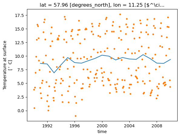
  intake_esm_dataset_key :

  CMIP.historical.CESM2.fx.gn

13.1 Resample

ds_yearly = ds_kristineberg.resample(time='YE').mean('time')

ds_yearly['T_C'].plot()
ds_kristineberg['T_C'].plot(linewidth=0, marker='.')

[<matplotlib.lines.Line2D at 0x7f7dc68b87a0>]

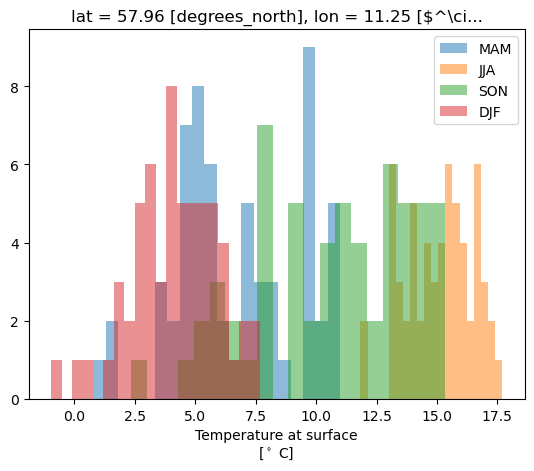
13.2 Filter data using .where():

ds_kristineberg['season'] = ds_kristineberg['time.season']

for s in ['MAM','JJA','SON','DJF']:
    ds_kristineberg.where(ds_kristineberg['season']==s)['T_C'].plot.hist(alpha=0.5, bins=20, label=s)
    
plt.legend()

<matplotlib.legend.Legend at 0x7f7dc68869c0>

13.3 Group by with .groupby()

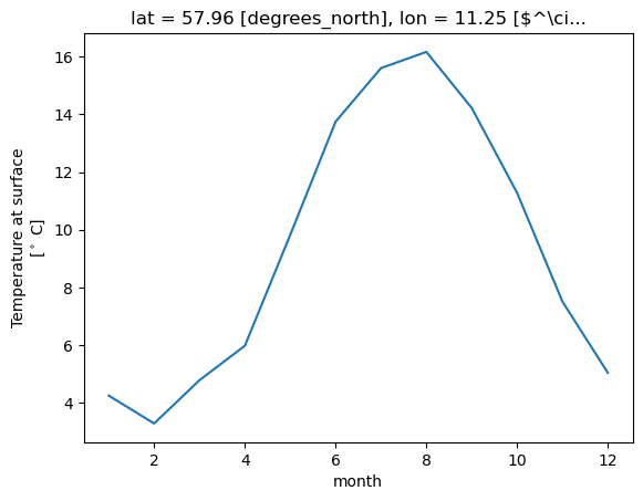
ds_kristineberg['month'] = ds_kristineberg['time.month']

ds_kristineberg

<xarray.Dataset> Size: 12kB
Dimensions:         (member_id: 1, dcpp_init_year: 1, time: 240, nbnd: 2)
Coordinates:
  * member_id       (member_id) object 8B 'r1i1p1f1'
  * dcpp_init_year  (dcpp_init_year) object 8B None
  * time            (time) datetime64[ns] 2kB 1990-01-15T12:00:00 ... 2009-12...
    lat             float64 8B 57.96
    lon             float64 8B 11.25
    a_bnds          (nbnd) float64 16B 0.005032 0.002255
    b_bnds          (nbnd) float64 16B 0.0 0.0
    lev             float64 8B -992.6
    lev_bnds        (nbnd) float64 16B 0.005032 0.002255
Dimensions without coordinates: nbnd
Data variables:
    areacella       (member_id, dcpp_init_year) float32 4B 7.728e+09
    a               float64 8B 0.0
    b               float64 8B 0.9926
    mmrso4          (member_id, dcpp_init_year, time) float32 960B 9.319e-10 ...
    p0              float32 4B 1e+05
    ps              (time) float32 960B 1.009e+05 9.98e+04 ... 1.001e+05
    hurs            (member_id, dcpp_init_year, time) float32 960B 85.65 ... ...
    tas             (member_id, dcpp_init_year, time) float32 960B 277.0 ... ...
    T_C             (member_id, dcpp_init_year, time) float32 960B 3.886 ... ...
    season          (time) <U3 3kB 'DJF' 'DJF' 'MAM' 'MAM' ... 'SON' 'SON' 'DJF'
    month           (time) int64 2kB 1 2 3 4 5 6 7 8 9 ... 4 5 6 7 8 9 10 11 12
Attributes: (12/58)
    Conventions:                      CF-1.7 CMIP-6.2
    activity_id:                      CMIP
    branch_method:                    standard
    branch_time_in_child:             674885.0
    branch_time_in_parent:            219000.0
    case_id:                          15
    ...                               ...
    intake_esm_attrs:variable_id:     areacella
    intake_esm_attrs:grid_label:      gn
    intake_esm_attrs:zstore:          gs://cmip6/CMIP6/CMIP/NCAR/CESM2/histor...
    intake_esm_attrs:version:         20190308
    intake_esm_attrs:_data_format_:   zarr
    intake_esm_dataset_key:           CMIP.historical.CESM2.fx.gn

xarray.Dataset

• Dimensions:
  • member_id: 1
  • dcpp_init_year: 1
  • time: 240
  • nbnd: 2
• Coordinates: (9)
  • member_id
    (member_id)
    object
    'r1i1p1f1'

    array(['r1i1p1f1'], dtype=object)

  • dcpp_init_year
    (dcpp_init_year)
    object
    None

    array([None], dtype=object)

  • time
    (time)
    datetime64[ns]
    1990-01-15T12:00:00 ... 2009-12-...

    array(['1990-01-15T12:00:00.000000000', '1990-02-14T00:00:00.000000000',
           '1990-03-15T12:00:00.000000000', ..., '2009-10-15T12:00:00.000000000',
           '2009-11-15T00:00:00.000000000', '2009-12-15T12:00:00.000000000'],
          shape=(240,), dtype='datetime64[ns]')

  • lat
    ()
    float64
    57.96

    axis :

    Y

    bounds :

    lat_bnds

    standard_name :

    latitude

    title :

    Latitude

    type :

    double

    units :

    degrees_north

    valid_max :

    90.0

    valid_min :

    -90.0

    array(57.95811518)

  • lon
    ()
    float64
    11.25

    axis :

    X

    bounds :

    lon_bnds

    standard_name :

    longitude

    title :

    Longitude

    type :

    double

    units :

    $^\circ$ East

    valid_max :

    360.0

    valid_min :

    0.0

    array(11.25)

  • a_bnds
    (nbnd)
    float64
    0.005032 0.002255

    long_name :

    vertical coordinate formula term: a(k+1/2)

    array([0.00503169, 0.00225524])

  • b_bnds
    (nbnd)
    float64
    0.0 0.0

    long_name :

    vertical coordinate formula term: b(k+1/2)

    array([0., 0.])

  • lev
    ()
    float64
    -992.6

    axis :

    Z

    bounds :

    lev_bnds

    positive :

    up

    standard_name :

    alevel

    title :

    atmospheric model level

    type :

    double

    units :

    hPa

    array(-992.55609512)

  • lev_bnds
    (nbnd)
    float64
    0.005032 0.002255

    formula :

    p = a*p0 + b*ps

    formula_terms :

    p0: p0 a: a_bnds b: b_bnds ps: ps

    standard_name :

    atmosphere_hybrid_sigma_pressure_coordinate

    units :

    hPa

    array([0.00503169, 0.00225524])

• Data variables: (11)
  • areacella
    (member_id, dcpp_init_year)
    float32
    7.728e+09

    cell_methods :

    area: sum

    comment :

    Cell areas for any grid used to report atmospheric variables and any other variable using that grid (e.g., soil moisture content). These cell areas should be defined to enable exact calculation of global integrals (e.g., of vertical fluxes of energy at the surface and top of the atmosphere).

    description :

    Cell areas for any grid used to report atmospheric variables and any other variable using that grid (e.g., soil moisture content). These cell areas should be defined to enable exact calculation of global integrals (e.g., of vertical fluxes of energy at the surface and top of the atmosphere).

    frequency :

    fx

    id :

    areacella

    long_name :

    Grid-Cell Area for Atmospheric Grid Variables

    mipTable :

    fx

    out_name :

    areacella

    prov :

    fx ((isd.003))

    realm :

    atmos land

    standard_name :

    cell_area

    time_label :

    None

    time_title :

    No temporal dimensions ... fixed field

    title :

    Grid-Cell Area for Atmospheric Grid Variables

    type :

    real

    units :

    m2

    variable_id :

    areacella

    array([[7.727901e+09]], dtype=float32)

  • a
    ()
    float64
    0.0

    bounds :

    a_bnds

    long_name :

    vertical coordinate formula term: a(k)

    array(0.)

  • b
    ()
    float64
    0.9926

    bounds :

    b_bnds

    long_name :

    vertical coordinate formula term: b(k)

    array(0.9925561)

  • mmrso4
    (member_id, dcpp_init_year, time)
    float32
    9.319e-10 9.139e-10 ... 4.485e-10

    cell_measures :

    area: areacella

    cell_methods :

    area: time: mean

    comment :

    Dry mass of sulfate (SO4) in aerosol particles as a fraction of air mass.

    description :

    Dry mass of sulfate (SO4) in aerosol particles as a fraction of air mass.

    frequency :

    mon

    id :

    mmrso4

    long_name :

    Aerosol Sulfate Mass Mixing Ratio

    mipTable :

    AERmon

    out_name :

    mmrso4

    prov :

    AERmon ((isd.003))

    realm :

    aerosol

    standard_name :

    mass_fraction_of_sulfate_dry_aerosol_particles_in_air

    time :

    time

    time_label :

    time-mean

    time_title :

    Temporal mean

    title :

    Aerosol Sulfate Mass Mixing Ratio

    type :

    real

    units :

    kg kg-1

    variable_id :

    mmrso4

    array([[[9.3193886e-10, 9.1392072e-10, 1.2826715e-09, 7.2257367e-10,
             2.2636457e-09, 1.3281619e-09, 1.4629278e-09, 1.2863141e-09,
             6.4677341e-10, 1.5266306e-09, 9.0736763e-10, 5.7557659e-10,
             4.7942467e-10, 7.3377227e-10, 1.9957693e-09, 1.4964732e-09,
             1.2506074e-09, 1.6712218e-09, 1.3250209e-09, 1.6674845e-09,
             3.6972247e-10, 5.6149579e-10, 7.6491025e-10, 1.6698171e-09,
             9.8607511e-10, 6.4137351e-10, 7.8463064e-10, 1.2971688e-09,
             1.1532616e-09, 1.2129736e-09, 1.2082786e-09, 1.2557465e-09,
             6.2253258e-10, 5.0003912e-10, 3.1542999e-10, 6.8933742e-10,
             7.3369416e-10, 6.5658307e-10, 5.3543248e-10, 4.7376575e-10,
             1.0168403e-09, 1.6001662e-09, 4.8634125e-10, 8.9594443e-10,
             2.1212649e-09, 3.1811920e-10, 3.5666189e-10, 1.3520196e-09,
             5.6667299e-10, 5.1949695e-10, 4.2386877e-10, 1.4821199e-09,
             1.4134094e-09, 1.3894664e-09, 1.0615168e-09, 1.5850201e-09,
             1.1513889e-09, 6.5186895e-10, 1.1817154e-09, 7.4557799e-10,
             1.9564568e-09, 7.6402235e-10, 7.2592093e-10, 5.3814297e-10,
             1.7240011e-09, 1.4250184e-09, 1.2221594e-09, 6.8972605e-10,
             6.9383221e-10, 1.2773098e-09, 4.0283718e-10, 3.9811388e-10,
             9.7333863e-10, 4.4941270e-10, 5.5883020e-10, 1.2838162e-09,
             1.2748105e-09, 1.1566451e-09, 8.2630669e-10, 1.3249776e-09,
    ...
             7.5434198e-10, 3.2416719e-10, 6.7540507e-10, 5.2173044e-10,
             1.6671606e-10, 2.1651315e-10, 2.7970151e-10, 3.9993286e-10,
             8.1241042e-10, 1.0122931e-09, 4.2739132e-10, 6.4456152e-10,
             3.5591874e-10, 4.1421538e-10, 3.1068517e-10, 2.5002367e-10,
             3.2186834e-10, 2.1786670e-10, 6.5897471e-10, 5.5566390e-10,
             8.8390589e-10, 5.5829497e-10, 8.0862272e-10, 4.4708118e-10,
             4.1382620e-10, 8.7374258e-10, 6.8856332e-10, 2.2117561e-10,
             5.1323434e-10, 3.2079947e-10, 4.4620288e-10, 4.8293736e-10,
             8.8299312e-10, 1.1971121e-09, 7.2521211e-10, 4.9940829e-10,
             5.3397714e-10, 6.6344513e-10, 4.7186260e-10, 1.6243321e-10,
             3.7509162e-10, 7.4617806e-10, 5.9407895e-10, 4.0051451e-10,
             1.1766452e-09, 6.6410638e-10, 7.5369005e-10, 7.0132800e-10,
             6.3694217e-10, 3.4894496e-10, 1.8863487e-10, 4.3067430e-10,
             2.1598053e-10, 2.9836339e-10, 3.3995992e-10, 8.6714907e-10,
             2.7420552e-10, 5.7396254e-10, 7.0535694e-10, 5.1266724e-10,
             5.1790988e-10, 4.0158260e-10, 3.3728587e-10, 7.2649092e-10,
             9.6747377e-10, 2.6640706e-10, 4.2341586e-10, 3.3404060e-10,
             8.1849499e-10, 4.7471893e-10, 5.2741644e-10, 6.4691424e-10,
             6.1747668e-10, 5.2262034e-10, 2.4114855e-10, 4.4853779e-10]]],
          dtype=float32)

  • p0
    ()
    float32
    1e+05

    long_name :

    vertical coordinate formula term: reference pressure

    units :

    Pa

    array(100000., dtype=float32)

  • ps
    (time)
    float32
    1.009e+05 9.98e+04 ... 1.001e+05

    long_name :

    surface_air_pressure

    units :

    Pa

    array([100904.234,  99803.57 , 100440.516, 100448.22 , 100559.37 ,
           100523.586, 100212.87 , 100926.34 , 100852.14 , 102373.44 ,
            99654.45 ,  99055.27 , 100831.14 , 101204.37 , 100669.15 ,
           101525.4  , 100658.04 , 100938.45 , 100765.89 , 100344.7  ,
           101106.18 , 100046.78 , 100264.36 , 101182.875,  99921.31 ,
           100148.945, 100310.14 , 101481.36 , 100976.25 , 101004.67 ,
           100595.63 , 101399.23 , 100775.016,  99661.59 , 100557.336,
           100853.5  , 100602.05 ,  99416.125,  99361.98 , 100562.04 ,
           101226.49 , 100736.195, 100330.27 , 100303.45 , 101486.32 ,
           100172.08 ,  99968.98 ,  99555.11 ,  99927.11 , 100957.336,
           102040.26 , 100934.12 , 100969.86 , 101089.08 , 100895.67 ,
           100699.11 , 101067.555, 100813.62 , 100003.445, 100423.6  ,
           100467.21 , 100953.91 , 100940.54 , 100775.586, 100702.66 ,
           101299.7  , 100351.016, 100299.23 , 100356.16 , 101226.16 ,
            99500.45 , 100647.055,  99774.76 ,  99729.57 , 101999.5  ,
           101972.29 , 100723.21 , 101099.19 ,  99999.555, 101058.45 ,
           100691.75 , 101163.89 , 100137.19 ,  99852.35 , 100074.82 ,
            99509.35 , 101196.   , 100173.195, 100193.29 , 100543.4  ,
           100037.92 ,  99772.36 , 101303.164, 101312.016, 100387.48 ,
            99350.48 , 100342.07 , 100571.6  , 100091.83 ,  99747.67 ,
    ...
           100339.91 , 100146.95 , 100370.82 , 100408.83 , 101103.51 ,
           100334.51 , 101051.38 , 100733.7  , 100076.39 ,  99451.71 ,
            99377.695, 100538.17 ,  99619.125, 101456.266, 100809.23 ,
           100892.445, 101035.05 , 100955.49 , 101370.05 , 101036.4  ,
           100480.266, 100232.76 , 100793.11 , 100296.17 ,  99655.34 ,
           100817.61 , 101024.12 , 101460.71 , 100830.484,  99863.086,
           100603.45 , 100615.73 , 100579.125,  99717.32 ,  99928.   ,
            99814.71 ,  98976.21 , 100500.06 , 100021.984, 100716.84 ,
           100708.6  , 100666.12 , 100306.61 , 100505.89 , 101491.58 ,
           100169.445, 100272.66 , 101319.055, 100523.24 ,  99671.836,
           101458.9  , 100630.016, 100541.26 , 100431.43 , 101172.04 ,
           100969.13 , 101572.61 ,  99554.836,  98949.96 , 100866.375,
           101577.19 , 100174.56 , 100970.914, 101222.98 , 100652.19 ,
            99996.75 , 101146.86 , 101189.18 ,  99726.875,  99874.49 ,
            99992.64 ,  99526.875,  99982.586, 100155.43 , 100541.37 ,
           101167.44 , 100320.7  , 100911.055, 100909.5  , 100727.58 ,
            99840.336, 100138.62 , 101668.38 , 101567.586,  99259.99 ,
           101204.73 , 101241.016, 100997.39 , 100652.47 , 100954.375,
           101550.71 , 101144.49 ,  99947.56 , 100891.67 , 100086.77 ],
          dtype=float32)

  • hurs
    (member_id, dcpp_init_year, time)
    float32
    85.65 79.78 82.47 ... 83.64 89.49

    cell_measures :

    area: areacella

    cell_methods :

    area: time: mean

    comment :

    This is the relative humidity with respect to liquid water for T> 0 C, and with respect to ice for T<0 C.

    description :

    This is the relative humidity with respect to liquid water for T> 0 C, and with respect to ice for T<0 C.

    frequency :

    mon

    id :

    hurs

    long_name :

    Near-Surface Relative Humidity

    mipTable :

    Amon

    out_name :

    hurs

    prov :

    Amon ((isd.003))

    realm :

    atmos

    standard_name :

    relative_humidity

    time :

    time

    time_label :

    time-mean

    time_title :

    Temporal mean

    title :

    Near-Surface Relative Humidity

    type :

    real

    units :

    %

    variable_id :

    hurs

    array([[[85.6512  , 79.7797  , 82.473785, 79.58873 , 80.421875,
             84.58708 , 84.94299 , 72.892365, 75.627266, 83.52159 ,
             81.26038 , 84.68246 , 81.28056 , 86.9214  , 84.940254,
             71.434   , 81.14642 , 84.55596 , 79.76721 , 82.525185,
             69.615944, 77.52233 , 79.28391 , 89.902054, 89.68583 ,
             86.76022 , 78.673225, 80.402504, 77.28582 , 86.062775,
             84.12753 , 81.188934, 72.5107  , 78.06689 , 79.50622 ,
             85.14791 , 85.16971 , 79.308556, 81.106255, 74.15938 ,
             76.85091 , 83.09885 , 80.1934  , 77.61525 , 81.34912 ,
             74.56923 , 81.82556 , 86.91707 , 84.77872 , 79.13002 ,
             70.701294, 76.79796 , 81.3291  , 81.01642 , 84.95078 ,
             80.43662 , 78.639725, 79.71097 , 82.36563 , 82.5781  ,
             86.097916, 77.24076 , 84.35341 , 76.216255, 82.4589  ,
             83.908615, 81.38897 , 79.03039 , 76.288734, 81.49444 ,
             83.08849 , 81.42568 , 88.53188 , 85.09241 , 77.77556 ,
             79.70282 , 80.305466, 83.2992  , 80.25415 , 81.289894,
             80.31601 , 86.42468 , 79.22198 , 80.783966, 85.659645,
             82.79457 , 83.75577 , 83.89612 , 87.54124 , 85.52979 ,
             84.52526 , 78.82385 , 83.94702 , 80.09471 , 82.58052 ,
             85.81947 , 88.3496  , 81.24771 , 81.73555 , 80.737564,
    ...
             86.58703 , 77.65002 , 76.92285 , 82.098526, 81.421104,
             81.656944, 85.26446 , 76.72732 , 78.53415 , 84.1566  ,
             83.29057 , 81.94568 , 78.68756 , 75.4941  , 73.73777 ,
             83.86288 , 83.008995, 80.959   , 78.48728 , 77.348274,
             76.765884, 82.4043  , 84.123245, 84.66348 , 77.667564,
             80.34306 , 74.82629 , 81.81224 , 84.970146, 80.859344,
             80.14923 , 73.6474  , 82.12172 , 83.96776 , 83.2338  ,
             83.37189 , 81.97976 , 77.62364 , 84.172966, 84.03998 ,
             79.95671 , 84.44249 , 76.10524 , 79.596825, 81.99454 ,
             85.85605 , 80.008606, 80.301796, 83.00442 , 82.715614,
             77.42871 , 81.817406, 86.23183 , 81.13182 , 81.60189 ,
             75.99792 , 80.1371  , 81.668274, 80.24692 , 85.04006 ,
             85.7113  , 83.677536, 69.43945 , 83.40899 , 83.40006 ,
             85.41751 , 84.303856, 77.21337 , 77.8262  , 76.52623 ,
             82.73933 , 86.96575 , 83.560455, 79.949036, 78.34009 ,
             71.88216 , 82.32212 , 82.4355  , 77.32013 , 80.14359 ,
             80.89918 , 79.335236, 84.31219 , 89.36123 , 84.628136,
             79.660576, 71.35938 , 79.27945 , 82.85541 , 79.48341 ,
             82.33854 , 75.105225, 81.02953 , 83.64138 , 89.48721 ]]],
          dtype=float32)

  • tas
    (member_id, dcpp_init_year, time)
    float32
    277.0 273.6 277.4 ... 278.7 277.5

    cell_measures :

    area: areacella

    cell_methods :

    area: time: mean

    comment :

    near-surface (usually, 2 meter) air temperature

    description :

    near-surface (usually, 2 meter) air temperature

    frequency :

    mon

    id :

    tas

    long_name :

    Near-Surface Air Temperature

    mipTable :

    Amon

    out_name :

    tas

    prov :

    Amon ((isd.003))

    realm :

    atmos

    standard_name :

    air_temperature

    time :

    time

    time_label :

    time-mean

    time_title :

    Temporal mean

    title :

    Near-Surface Air Temperature

    type :

    real

    units :

    K

    variable_id :

    tas

    array([[[277.036  , 273.6018 , 277.4057 , 280.13733, 283.04315,
             286.1976 , 288.96158, 288.67313, 286.447  , 282.331  ,
             280.6072 , 277.33212, 276.35056, 275.45718, 278.24026,
             278.6902 , 282.02042, 287.577  , 289.411  , 289.88937,
             286.20694, 283.30524, 278.37958, 274.88986, 275.9685 ,
             273.18692, 273.93338, 277.60355, 280.31152, 285.03375,
             287.31808, 288.47113, 285.9238 , 282.57498, 275.49026,
             275.0295 , 277.4612 , 276.80396, 278.17105, 278.80664,
             281.17633, 286.22424, 286.43982, 286.2223 , 286.87054,
             280.75034, 281.23383, 278.1589 , 279.02744, 276.0177 ,
             274.74112, 278.6569 , 282.93082, 286.23575, 290.3751 ,
             289.93   , 287.68118, 285.75076, 282.43347, 280.83716,
             276.75778, 274.70197, 277.61902, 279.36847, 282.76617,
             286.89862, 287.75464, 288.02655, 286.36737, 283.76627,
             281.2449 , 278.22116, 275.7414 , 272.185  , 274.5559 ,
             278.77332, 282.7405 , 287.1005 , 287.9257 , 289.6798 ,
             287.99744, 285.52274, 282.72733, 277.2558 , 275.17532,
             277.2748 , 278.09113, 280.724  , 283.00928, 286.29123,
             288.06375, 288.2159 , 288.11716, 282.65875, 280.7434 ,
             279.24933, 279.11615, 277.5452 , 277.96658, 280.3044 ,
    ...
             276.63882, 278.0943 , 278.8853 , 282.86172, 286.525  ,
             288.575  , 290.84235, 287.7864 , 286.16046, 282.43958,
             278.81308, 277.3345 , 277.58786, 276.546  , 278.729  ,
             283.8123 , 287.2157 , 289.00388, 290.0209 , 288.48395,
             284.43906, 280.91425, 277.32306, 277.92804, 276.23212,
             277.96164, 279.61298, 283.68323, 287.7096 , 288.3466 ,
             289.01794, 286.41257, 283.7271 , 279.47147, 280.5569 ,
             279.27786, 279.0786 , 278.42728, 280.98596, 284.1375 ,
             286.53778, 289.71893, 289.15417, 287.5555 , 284.9453 ,
             282.5847 , 278.54913, 276.3146 , 276.473  , 278.11572,
             281.2289 , 283.62564, 287.56595, 288.81967, 289.9035 ,
             287.19138, 284.7344 , 280.03235, 278.63467, 275.95413,
             276.34845, 276.56122, 276.8956 , 282.77957, 287.18732,
             288.75058, 290.00266, 288.32962, 283.43085, 280.71335,
             275.38644, 277.57248, 275.94055, 277.2333 , 278.06137,
             281.24808, 284.98416, 288.2797 , 289.20377, 286.846  ,
             284.86862, 279.29944, 278.14166, 278.26358, 277.8097 ,
             278.3669 , 277.93552, 283.2631 , 286.61642, 288.55844,
             290.29236, 288.50214, 284.51822, 278.70798, 277.5374 ]]],
          dtype=float32)

  • T_C
    (member_id, dcpp_init_year, time)
    float32
    3.886 0.4518 4.256 ... 5.558 4.387

    cell_measures :

    area: areacella

    cell_methods :

    area: time: mean

    comment :

    near-surface (usually, 2 meter) air temperature

    description :

    near-surface (usually, 2 meter) air temperature

    frequency :

    mon

    id :

    tas

    long_name :

    Temperature at surface

    mipTable :

    Amon

    out_name :

    tas

    prov :

    Amon ((isd.003))

    realm :

    atmos

    standard_name :

    air_temperature

    time :

    time

    time_label :

    time-mean

    time_title :

    Temporal mean

    title :

    Near-Surface Air Temperature

    type :

    real

    units :

    $^\circ$ C

    variable_id :

    tas

    array([[[ 3.8860168 ,  0.45181274,  4.255707  ,  6.987335  ,
              9.893158  , 13.047607  , 15.811584  , 15.523132  ,
             13.296997  ,  9.181     ,  7.4572144 ,  4.182129  ,
              3.2005615 ,  2.30719   ,  5.090271  ,  5.5401917 ,
              8.870422  , 14.427002  , 16.261017  , 16.73938   ,
             13.056946  , 10.155243  ,  5.2295837 ,  1.7398682 ,
              2.818512  ,  0.03692627,  0.78338623,  4.4535522 ,
              7.1615295 , 11.883759  , 14.168091  , 15.321136  ,
             12.773804  ,  9.424988  ,  2.340271  ,  1.8795166 ,
              4.3112183 ,  3.6539612 ,  5.021057  ,  5.6566467 ,
              8.026337  , 13.074249  , 13.289825  , 13.072296  ,
             13.720551  ,  7.600342  ,  8.083832  ,  5.008911  ,
              5.8774414 ,  2.8677063 ,  1.5911255 ,  5.506897  ,
              9.780823  , 13.085754  , 17.225098  , 16.779999  ,
             14.531189  , 12.600769  ,  9.283478  ,  7.6871643 ,
              3.607788  ,  1.5519714 ,  4.4690247 ,  6.2184753 ,
              9.61618   , 13.748627  , 14.604645  , 14.876556  ,
             13.217377  , 10.616272  ,  8.09491   ,  5.071167  ,
              2.5914001 , -0.96499634,  1.4059143 ,  5.6233215 ,
              9.590515  , 13.9505005 , 14.775696  , 16.529816  ,
    ...
             15.333954  , 11.2890625 ,  7.7642517 ,  4.173065  ,
              4.7780457 ,  3.0821228 ,  4.8116455 ,  6.462982  ,
             10.533234  , 14.559601  , 15.196594  , 15.86795   ,
             13.262573  , 10.577118  ,  6.321472  ,  7.406891  ,
              6.1278687 ,  5.9286194 ,  5.2772827 ,  7.835968  ,
             10.987518  , 13.387787  , 16.56894   , 16.00418   ,
             14.405518  , 11.795319  ,  9.434692  ,  5.3991394 ,
              3.1646118 ,  3.322998  ,  4.9657288 ,  8.078918  ,
             10.475647  , 14.415955  , 15.669678  , 16.75351   ,
             14.041382  , 11.584412  ,  6.8823547 ,  5.48468   ,
              2.8041382 ,  3.1984558 ,  3.4112244 ,  3.7456055 ,
              9.629578  , 14.037323  , 15.600586  , 16.852661  ,
             15.179626  , 10.280853  ,  7.5633545 ,  2.2364502 ,
              4.4224854 ,  2.7905579 ,  4.083313  ,  4.911377  ,
              8.0980835 , 11.8341675 , 15.1297    , 16.053772  ,
             13.696014  , 11.718628  ,  6.1494446 ,  4.9916687 ,
              5.1135864 ,  4.6596985 ,  5.216919  ,  4.7855225 ,
             10.113098  , 13.466431  , 15.408447  , 17.142365  ,
             15.352142  , 11.368225  ,  5.5579834 ,  4.3874207 ]]],
          dtype=float32)

  • season
    (time)
    <U3
    'DJF' 'DJF' 'MAM' ... 'SON' 'DJF'

    array(['DJF', 'DJF', 'MAM', 'MAM', 'MAM', 'JJA', 'JJA', 'JJA', 'SON',
           'SON', 'SON', 'DJF', 'DJF', 'DJF', 'MAM', 'MAM', 'MAM', 'JJA',
           'JJA', 'JJA', 'SON', 'SON', 'SON', 'DJF', 'DJF', 'DJF', 'MAM',
           'MAM', 'MAM', 'JJA', 'JJA', 'JJA', 'SON', 'SON', 'SON', 'DJF',
           'DJF', 'DJF', 'MAM', 'MAM', 'MAM', 'JJA', 'JJA', 'JJA', 'SON',
           'SON', 'SON', 'DJF', 'DJF', 'DJF', 'MAM', 'MAM', 'MAM', 'JJA',
           'JJA', 'JJA', 'SON', 'SON', 'SON', 'DJF', 'DJF', 'DJF', 'MAM',
           'MAM', 'MAM', 'JJA', 'JJA', 'JJA', 'SON', 'SON', 'SON', 'DJF',
           'DJF', 'DJF', 'MAM', 'MAM', 'MAM', 'JJA', 'JJA', 'JJA', 'SON',
           'SON', 'SON', 'DJF', 'DJF', 'DJF', 'MAM', 'MAM', 'MAM', 'JJA',
           'JJA', 'JJA', 'SON', 'SON', 'SON', 'DJF', 'DJF', 'DJF', 'MAM',
           'MAM', 'MAM', 'JJA', 'JJA', 'JJA', 'SON', 'SON', 'SON', 'DJF',
           'DJF', 'DJF', 'MAM', 'MAM', 'MAM', 'JJA', 'JJA', 'JJA', 'SON',
           'SON', 'SON', 'DJF', 'DJF', 'DJF', 'MAM', 'MAM', 'MAM', 'JJA',
           'JJA', 'JJA', 'SON', 'SON', 'SON', 'DJF', 'DJF', 'DJF', 'MAM',
           'MAM', 'MAM', 'JJA', 'JJA', 'JJA', 'SON', 'SON', 'SON', 'DJF',
           'DJF', 'DJF', 'MAM', 'MAM', 'MAM', 'JJA', 'JJA', 'JJA', 'SON',
           'SON', 'SON', 'DJF', 'DJF', 'DJF', 'MAM', 'MAM', 'MAM', 'JJA',
           'JJA', 'JJA', 'SON', 'SON', 'SON', 'DJF', 'DJF', 'DJF', 'MAM',
           'MAM', 'MAM', 'JJA', 'JJA', 'JJA', 'SON', 'SON', 'SON', 'DJF',
           'DJF', 'DJF', 'MAM', 'MAM', 'MAM', 'JJA', 'JJA', 'JJA', 'SON',
           'SON', 'SON', 'DJF', 'DJF', 'DJF', 'MAM', 'MAM', 'MAM', 'JJA',
           'JJA', 'JJA', 'SON', 'SON', 'SON', 'DJF', 'DJF', 'DJF', 'MAM',
           'MAM', 'MAM', 'JJA', 'JJA', 'JJA', 'SON', 'SON', 'SON', 'DJF',
           'DJF', 'DJF', 'MAM', 'MAM', 'MAM', 'JJA', 'JJA', 'JJA', 'SON',
           'SON', 'SON', 'DJF', 'DJF', 'DJF', 'MAM', 'MAM', 'MAM', 'JJA',
           'JJA', 'JJA', 'SON', 'SON', 'SON', 'DJF'], dtype='<U3')

  • month
    (time)
    int64
    1 2 3 4 5 6 7 ... 6 7 8 9 10 11 12

    array([ 1,  2,  3,  4,  5,  6,  7,  8,  9, 10, 11, 12,  1,  2,  3,  4,  5,
            6,  7,  8,  9, 10, 11, 12,  1,  2,  3,  4,  5,  6,  7,  8,  9, 10,
           11, 12,  1,  2,  3,  4,  5,  6,  7,  8,  9, 10, 11, 12,  1,  2,  3,
            4,  5,  6,  7,  8,  9, 10, 11, 12,  1,  2,  3,  4,  5,  6,  7,  8,
            9, 10, 11, 12,  1,  2,  3,  4,  5,  6,  7,  8,  9, 10, 11, 12,  1,
            2,  3,  4,  5,  6,  7,  8,  9, 10, 11, 12,  1,  2,  3,  4,  5,  6,
            7,  8,  9, 10, 11, 12,  1,  2,  3,  4,  5,  6,  7,  8,  9, 10, 11,
           12,  1,  2,  3,  4,  5,  6,  7,  8,  9, 10, 11, 12,  1,  2,  3,  4,
            5,  6,  7,  8,  9, 10, 11, 12,  1,  2,  3,  4,  5,  6,  7,  8,  9,
           10, 11, 12,  1,  2,  3,  4,  5,  6,  7,  8,  9, 10, 11, 12,  1,  2,
            3,  4,  5,  6,  7,  8,  9, 10, 11, 12,  1,  2,  3,  4,  5,  6,  7,
            8,  9, 10, 11, 12,  1,  2,  3,  4,  5,  6,  7,  8,  9, 10, 11, 12,
            1,  2,  3,  4,  5,  6,  7,  8,  9, 10, 11, 12,  1,  2,  3,  4,  5,
            6,  7,  8,  9, 10, 11, 12,  1,  2,  3,  4,  5,  6,  7,  8,  9, 10,
           11, 12])

• Attributes: (58)

  Conventions :

  CF-1.7 CMIP-6.2

  activity_id :

  CMIP

  branch_method :

  standard

  branch_time_in_child :

  674885.0

  branch_time_in_parent :

  219000.0

  case_id :

  15

  cesm_casename :

  b.e21.BHIST.f09_g17.CMIP6-historical.001

  contact :

  cesm_cmip6@ucar.edu

  creation_date :

  2019-01-16T21:43:39Z

  data_specs_version :

  01.00.29

  experiment :

  all-forcing simulation of the recent past

  experiment_id :

  historical

  forcing_index :

  1

  frequency :

  fx

  further_info_url :

  https://furtherinfo.es-doc.org/CMIP6.NCAR.CESM2.historical.none.r1i1p1f1

  grid :

  native 0.9x1.25 finite volume grid (192x288 latxlon)

  grid_label :

  gn

  initialization_index :

  1

  institution :

  National Center for Atmospheric Research, Climate and Global Dynamics Laboratory, 1850 Table Mesa Drive, Boulder, CO 80305, USA

  institution_id :

  NCAR

  license :

  CMIP6 model data produced by <The National Center for Atmospheric Research> is licensed under a Creative Commons Attribution-[]ShareAlike 4.0 International License (https://creativecommons.org/licenses/). Consult https://pcmdi.llnl.gov/CMIP6/TermsOfUse for terms of use governing CMIP6 output, including citation requirements and proper acknowledgment. Further information about this data, including some limitations, can be found via the further_info_url (recorded as a global attribute in this file)[]. The data producers and data providers make no warranty, either express or implied, including, but not limited to, warranties of merchantability and fitness for a particular purpose. All liabilities arising from the supply of the information (including any liability arising in negligence) are excluded to the fullest extent permitted by law.

  mip_era :

  CMIP6

  model_doi_url :

  https://doi.org/10.5065/D67H1H0V

  nominal_resolution :

  100 km

  parent_activity_id :

  CMIP

  parent_experiment_id :

  piControl

  parent_mip_era :

  CMIP6

  parent_source_id :

  CESM2

  parent_time_units :

  days since 0001-01-01 00:00:00

  parent_variant_label :

  r1i1p1f1

  physics_index :

  1

  product :

  model-output

  realization_index :

  1

  realm :

  atmos land

  source :

  CESM2 (2017): atmosphere: CAM6 (0.9x1.25 finite volume grid; 288 x 192 longitude/latitude; 32 levels; top level 2.25 mb); ocean: POP2 (320x384 longitude/latitude; 60 levels; top grid cell 0-10 m); sea_ice: CICE5.1 (same grid as ocean); land: CLM5 0.9x1.25 finite volume grid; 288 x 192 longitude/latitude; 32 levels; top level 2.25 mb); aerosol: MAM4 (0.9x1.25 finite volume grid; 288 x 192 longitude/latitude; 32 levels; top level 2.25 mb); atmoschem: MAM4 (0.9x1.25 finite volume grid; 288 x 192 longitude/latitude; 32 levels; top level 2.25 mb); landIce: CISM2.1; ocnBgchem: MARBL (320x384 longitude/latitude; 60 levels; top grid cell 0-10 m)

  source_id :

  CESM2

  source_type :

  AOGCM BGC

  sub_experiment :

  none

  sub_experiment_id :

  none

  table_id :

  fx

  tracking_id :

  hdl:21.14100/75033260-7bd2-46b9-9d98-3456f176d588

  variable_id :

  areacella

  variant_info :

  CMIP6 20th century experiments (1850-2014) with CAM6, interactive land (CLM5), coupled ocean (POP2) with biogeochemistry (MARBL), interactive sea ice (CICE5.1), and non-evolving land ice (CISM2.1)

  variant_label :

  r1i1p1f1

  status :

  2019-10-25;created;by nhn2@columbia.edu

  intake_esm_vars :

  ['areacella']

  intake_esm_attrs:activity_id :

  CMIP

  intake_esm_attrs:institution_id :

  NCAR

  intake_esm_attrs:source_id :

  CESM2

  intake_esm_attrs:experiment_id :

  historical

  intake_esm_attrs:member_id :

  r1i1p1f1

  intake_esm_attrs:table_id :

  fx

  intake_esm_attrs:variable_id :

  areacella

  intake_esm_attrs:grid_label :

  gn

  intake_esm_attrs:zstore :

  gs://cmip6/CMIP6/CMIP/NCAR/CESM2/historical/r1i1p1f1/fx/areacella/gn/v20190308/

  intake_esm_attrs:version :

  20190308

  intake_esm_attrs:_data_format_ :

  zarr

  intake_esm_dataset_key :

  CMIP.historical.CESM2.fx.gn

(ds_kristineberg['T_C']
    .groupby(ds_kristineberg['month'])
    .median()
    .plot()
)

[<matplotlib.lines.Line2D at 0x7f7dc504e5d0>]

14. Convert to pandas & do some random fun stuff:

Maybe we e.g. want to compare with a station, or just use some of the considerable functionalities available from pandas. It’s easy to convert back and forth between xarray and pandas:

A lot of these functions also exist in xarray!

Obs: might want to convert to pandas

At this point we basically have a time series and the dataset is not to big, so might want to convert to pandas:

subset_of_variables = ['mmrso4','hurs','tas','T_C','season']
df_kristineberg = ds_kristineberg[subset_of_variables].squeeze().to_dataframe()
df_kristineberg

lets do something unnecesarily complicated :D

Convert to pandas dataframe

Because more functionality

df = dss.isel(lev=-1)[vl].to_dataframe()

df_ri = df.reset_index()
df_ri.head()

qcut, cut

qcut splits the data into quantile ranges

df_ri['hurs_cat'] = pd.qcut(df_ri['hurs'],
                            q=[0.05,0.17, 0.34,0.66, 0.83,0.95],
                            labels=['very low','low','med','high','very high'],
                           )

Cut cuts into categories

df_ri['lat_cat'] = pd.cut(df_ri['lat'], [-90,-60,-30,0,30,60,90], 
                          labels=['S polar','S mid','S tropics', 'N tropic', 'N mid','N polar'])

df_ri

df_ri.sample(n=20000).groupby('lat_cat').mean(numeric_only=True)

sns.boxenplot(x="lat_cat", y="hurs",
              color="b",
              #scale="linear", 
              width_method='linear',
              data=df_ri)#.sample(n=20000))

sns.boxenplot(x="hurs_cat", 
              y="mmrso4",
              color="b",
              width_method='linear',
              data=df_ri.sample(n=20000),
             )

sns.displot(x="mmrso4",
            hue='lat_cat',
            log_scale=True,
            kind='kde',
            data=df_ri.sample(n=20000), 
            multiple="stack"
           )

Convert back to xarray if we need:

ds_new = df_ri.set_index(['time','lat','lon']).to_xarray()

ds_new

mask by category

ds_new.where(ds_new['hurs_cat']=='very low').mean(['time','lon'])['mmrso4'].plot(label='very low')#vmin = 0, vmax = 1.5e-8)
ds_new.where(ds_new['hurs_cat']=='low').mean(['time','lon'])['mmrso4'].plot(label='low')#vmin = 0, vmax = 1.5e-8)

ds_new.where(ds_new['hurs_cat']=='high').mean(['time','lon'])['mmrso4'].plot(label='high')#vmin = 0, vmax = 1.5e-8)
ds_new.where(ds_new['hurs_cat']=='very high').mean(['time','lon'], keep_attrs=True)['mmrso4'].plot(label='very high')#vmin = 0, vmax = 1.5e-8)
plt.legend()

Improve and reduce risk of typo:

for cat in ['very low','low','high','very high']:
    ds_new.where(ds_new['hurs_cat']==cat).mean(['time','lon'])['mmrso4'].plot(label=cat) 
plt.legend()